|
|
Home | Switchboard | Unix Administration | Red Hat | TCP/IP Networks | Neoliberalism | Toxic Managers |
| (slightly skeptical) Educational society promoting "Back to basics" movement against IT overcomplexity and bastardization of classic Unix | |||||||
|
|
As Hamlet observe during a different era "Something is rotten in the state of Denmark." It looks like the field now is ruled by the coalition of "complexity junkies" and "more cores is better" junkies.
Complexity of Kubernetes is such that even "bare-metal" installation of Kubernetes often is an overkill for HPC cluster and leads to waste of resources and slowing down of computations. So "classic" HPC configuration with scheduler still did not reached end of life point and such cluster are still competitive. Kubernetes initially was designed by Google as a load-balancing cluster, not as the HPC cluster.
Also more is not always better. The technical problems of serving, say, over 1K computational nodes from a single shared filesystem are tremendous. Scaling down cluster is often beneficial as due to Amdahl law (see below) almost no jobs benefit from running on, say, 512 cores and higher. And for such jobs there are GPUs, which in this case are a much better deal.
|
|
If "private cloud" solution is used situation is even worse and waste of resources and excessive complexity is higher. While container ecosystem is useful and solves some problems with Linux libraries (library hell) that exists in "classic" HPC clusters, the scope of those problems is small and does not justify losses in productivity and excessive complexity.
Classic HPC environment is based on two main components: common, shared filesystem and HPC scheduler. See for example
In the simplest form cluster is a set of nodes (each node is typical two socket server with higher end multicore CPU; although the high number of cores is not beneficial and even is detrimental for some application, for example for bioinformatics application and they can benefit form high clock speed of 4 core CPUs). For higher number of cores the problem of overheating is acute and requires water cooling solutions.
They are connected via high speed interconnect to server or servers that implement shared filesystem.
Grid computing is a broader term that cluster and typically refers to a set of (not necessary uniform like in cluster) servers connected to common scheduler, for example Sun Grid Engine and common storage. From this point of view HPC is a special case of grid computing
The key for HPC is the implementation of shares storage that allows functioning of a given number of nodes. A lot depends of the doman of application run on the cluster. many application do not require large shared storage to run, or they requre large storage to run but do not use MPI.
Two most common parallel filesystems currently used are Lustra and GPFS.
For larger number of nodes and if MPI is used Infiniband typically is used. For bioinformatics applications which do not use MPI Infiniband is not necessary, but is advisable because it improves the parameters of shared filesystem. GPFS can function directly on Infiniband layer without use of TCP/IP and that is a huge advantage for some applications.
Infiniband is a prerequisite for application that use MPI because of law latency but with the advent of 64 core CPUs (which means 128 core of two socket server and 256 threads if hyper threading is enabled ) the role of MPI to facilitate cross nodes communication is open to review. Truth be told MPI in HPC clusters is one of the most often abused subsystems because many researchers have no clue about optimum number of cores for their application and overspecify the number of cores several times, just because they can.
This situation is called "waiving dead chicken" and researchers working in computational chemistry (or "computational alchemistry;-) are typical members of the group that pracice this kind of abuse of HPC resources. Many of them have no or little clue about applications they use and they can get useful results form thier computations only by chance. Running jobs with large number of cores is a survival mechanism for them, no more no less. In general usefulness of many results in computational chemistry obtained on HPC clusters is subject to review ;-) .
I would like to stress that along with large memory nodes servers with high CPU clock speed (over 4GHz) are also legoitimate member of HPC sluters and shoudl be provided to researchers. Many genomic applications are single threaded and for such applicatins you do not need two socket server -- a single four or eight core CPUs with high clock frequency are much better then multicore monsters that Intel heavily pushed now. Often genomic job are running perfectly well on one socket workstation and buying for them two socket server is complete idiotism, which actually flourishes in modern organizations run by bean counters.
In this sense the current trend toward building clusters with most computational nodes using CPU with close to max available cores is a fallacy. Expensive fallacy. Cluster should be specialized for the set of applications it predominantly handles and for each application sweet spot of the number of cores exists -- this number should the base for selection of the servers for non-MPI jobs. 64 core servers are attractive for PowerPoint presentation but in reality they have several fundamental problems with the architecture of PC-compatible (Intel/AMD) servers.
Heat dissipation of multi-core CPU is a serious engineering challenge. Starting from probably 32 cores only liquid cooling is more or less adequate. And often even it can be inadequate for large loads and one need some special engineering solutions for this problem. Intel is working on such solutions.
Overheating of cores of servers running computationally intensive jobs is a really serious problem for clusters build using compact form factor for servers such as blades from Dell or HP. The compact form factor has inadequate heat dissipation. As the result they overheat, efficiency drops and all gain from additional cores disappear.
For the same reason using VMware for HPC clusters is a fallacy as it tends to increase this effect. The same consideration is application to the servers using in the major cloud providers such as AWS and Azure -- for them too overheating is a problem but it is completely hidden from the view as you do not have access to the server logs.
Parallel programming (like all programming) is as much art as science, always leaving room for major design improvements and performance enhancements. Software and hardware should go hand in hand when it comes to achieving high performance on a cluster. Programs must be written to explicitly take advantage of the underlying hardware. For some algorithms this is possible. For other it is not.
Limiting the size of the cluster helps as in smaller cluster parallel filesystem functions better and provides higher bandwidth to computational nodes.
Parallel programming mostly is limited to a certain subclass of computational algorithms Many algorithms can't be made parallel beyond relatively small number of cores (say 4, 8 and 16). Even for those that can be paralyzed efficiently over this limit the time spend per core often increased after a certain number of cores ("saturation"). This effect is connected with so called Amdahl named after one of the "founding fathers" of IBM system/360 Gene Amdahl (thanks to him we have 8 bit byte and byte addressing), and was presented at the AFIPS Spring Joint Computer Conference in 1967. This effect is very pronounced for Accelrys, VASP and several other common commercial programs. Jobs for which often are run by clueless researchers with the excessive number of cores.
| Simplifying, Amhdal law postulates that that in most cases the theoretical speedup from parallelization is limited to 20 times the single thread performance no matter how many CPUs you use. |
Suppose 1/N of the total time taken by a program in a part that can not be parallelized, and the rest (1-1/N) is in the parallelizable part. In this case the speedup always has a distinct "saturation" point and is governed by the following curves (see Amdahl's law - Wikipedia). Simplifying it postulates that that in most cases the theoretical speedup is limited to 20 times the single thread performance:
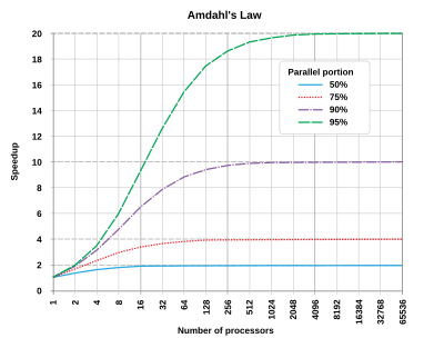
In theory you could apply an infinite amount of hardware to do the parallel part in zero time, but the sequential part will see no improvements. As a result, the best you can achieve is to execute the program in 1/N of the original time, but no faster. In parallel programming, this fact is commonly referred to as Amdahl's Law.
Amdahl's Law governs the speedup of using N parallel processors on a problem versus using only one serial processor. Speedup is defined as the time it takes a program to execute in serial (with one processor) divided by the time it takes to execute in parallel (with many processors):
     T(1)
S = ------
     T(j)
Where T(j) is the time it takes to execute the program when using j processors.
The real hard work in writing a parallel program is to make N as large as possible. But there is an interesting twist to it. You normally attempt bigger problems on more powerful computers, and usually the proportion of the time spent on the sequential parts of the code decreases with increasing problem size (as you tend to modify the program and increase the parallelizable portion to optimize the available resources).
| Gigantomania (from Ancient Greek γίγας gigas, "giant" and μανία mania, "madness") is the production of unusually and superfluously large works.[1] Gigantomania is in varying degrees a feature of the political and cultural lives of prehistoric and ancient civilizations (Megalithic cultures, Ancient Egypt, Ancient Rome, Ancient China, Aztec civilization), several totalitarian regimes (Stalin's USSR, Nazi Germany, Fascist Italy, Maoist China, Juche Korea),[1] as well as of contemporary capitalist countries (notably for skyscrapers and shopping malls). |
Carefully hidden fact is that that Gigantomania rules the HPC space. First of all the criteria of measuring HPC cluster productively (petaflops measured using completely artificial for real cluster loads and infinitely scalable Linpack benchmark) is highly suspect and have little on nothing to do with real application running on many clusters.
In this sense TOP500 list is more strongly correlates with the level of influence of military industrial complex on the country leadership, not so much with the progress in building useful clusters (although along with modeling on nuclear explosions there are few application for example related to weather forecasts that benefit from very high parallelization of computations).
The of small clusters (way with less then 64 computational nodes) on which a lot useful work can be done is deprecated and in many organization that are completely eliminated although small clusters allow high bandwidth per computation nodes then larger cluster.
Clusters are built to perform massive computations, and you need to know how fast they are. Standard benchmark based on LINPACK calculations is completely bizarre and false measure in many areas but one: the class of applications with unlimited parallelism.
The real applications usually do not scale above, say 128 cores well and many does not scale above 32 cores. So megaflop value used for large cluster and in Top500 index is just "art for the sake of art" and has very little connection to reality. It is a completely fake measure that suggests that more nodes and more cores are better.
That far far from being true. If your application does not scale above say 16 node that only thing you can do is to run many instances of such application in parallel. Of course, this can have great value as you can put more dots on some curve in a single day running computation is slightly different sets of data filling the chosen interval that you need to explore. But you will never get a better duration of a single computation then of much more modest cluster, that cost tiny fraction (say 1/10th) of the supercluster cost.
IBM is one firm that propagated this nonsense with LINPACK as the key benchmark of cluster performance. This test is fake in a sense that it assumes unlimited parallelism:
Cluster is generally is as good as each single computational node and megoflops tent to push designed toward larger amount of cores per CPU, which is completely wrong approach. It's common to think that the processor frequency determines performance. While this is true to a certain extent, it is of little value in comparing processors from different vendors or even different processor families from the same vendor because different processors do different amounts of work in a given number of clock cycles. This was especially obvious when we compared vector processors with scalar processors (see Part 1). Speed of memory also matter.
A more natural way to compare performance is to run some standard tests. Over the years a test known as the LINPACK benchmark has become a gold standard when comparing performance of HPC clusters. It was written by Jack Dongarra more than a decade ago and is still used by top500.org (see Resources for a link).
This test involves solving a dense system of N linear equations, where the number of floating-point operations is known (of the order of N^3). This test is well suited to speed test computers meant to run scientific applications and simulations because they tend to solve linear equations at some stage or another.
The standard unit of measurement is the number of floating-point operations or flops per second (in this case, a flop is either an addition or a multiplication of a 64-bit number). The test measures the following:
- Rpeak, theoretical peak flops. In a June 2005 report, IBM Blue Gene/L clocks at 183.5 tflops (trillion flops).
- Nmax, the matrix size N that gives the highest flops. For Blue Gene this number is 1277951.
- Rmax, the flops attained for Nmax. For Blue Gene, this number is 136.8 tflops.
To appreciate these numbers, consider that IBM BlueGene/L can compute in one second that task that on your home computer may take up to five days.
This phrase "IBM BlueGene/L can compute in one second that task that on your home computer may take up to five days" is complete nonsense in view of the Amdahl law. Probably such applications exist, but they are very rare. Here IBM is simply dishonest.
Clearly, it is hard to maintain a very large cluster. It requires special subsystems such as cluster manager (For example Bright Computing cluster mananger). Everything becomes a problem. It is not convenient to copy files to every node, set up SSH and MPI on every node that gets added, make appropriate changes when a node is removed, and so on.
For small clusters such problem are several magnitude less. Moreover for small cluster you can reuse some integrated solution such as Rocks, which provides most of the things we need for the cluster and automate some of the typical tasks. When it comes to managing a cluster in a production environment with a large user base, job scheduling and monitoring are crucial.
They include
Sun grid engine (now Oracle grid engine) can be used a powerful scheduler for computational clusters. Another popular scheduling system is OpenPBS, and Torque. Using it you can create queues and submit jobs on them. Like SGE both have open source versions along with the commercial versions.
You can also create sophisticated job-scheduling policies.
All "grid" schedulers let you view executing jobs, submit jobs, and cancel jobs. It also allows control over the maximum amount of CPU time available to a particular job, which is quite useful for an administrator.
An important aspect of managing clusters is monitoring, especially if your cluster has a large number of nodes. Several options are available, such as Nagios or Ganglia
Ganglia has a Web-based front end and provides real-time monitoring for CPU and memory usage; you can easily extend it to monitor just about anything. For example, with simple scripts you can make Ganglia report on CPU temperatures, fan speeds, etc.
|
|
Switchboard | ||||
| Latest | |||||
| Past week | |||||
| Past month | |||||
Jun 30, 2021 | www.theregister.com
Companies rely on estimates that are often wrong, says CNCF Tim Anderson Tue 29 Jun 2021 // 16:28 UTC
20
A report on Kubernetes expenditure from the Cloud Native Computing Foundation (CNCF), in association with the FinOps Foundation, shows that costs are rising and companies struggle to predict them accurately.
The new report is based on a survey of the CNCF and FinOps Foundation communities and although it had only 195 respondents, there was a "strong enterprise representation".
Spending on Kubernetes was up, according to the survey, with 67 per cent reporting an increase of 20 per cent or more over the last 12 months, and 10 per cent spending more than $1m per month on their deployments.
Kubernetes, as Reg readers know, is a means of orchestrating containerised applications, so its actual cost is mainly that of the resources it consumes: over 80 per cent compute (such as VMs on AWS, GCP or Azure) and a bit on memory, storage, networking and so on.
What's the FinOps Foundation? The FinOps Foundation was set up in 2019 by Cloudability, a cloud financial management company now part of Aptio.In 2020 it became part of the Linux Foundation, alongside Kubernetes overseer Cloud Native Computing Foundation, and aims to "advance the discipline of cloud financial management." Sponsors include Aptio, Atlassian, VMware and Google Cloud.
Basically, it is a kind of alliance of those hoping to manage and reduce their cloud spend, including Nationwide, Spotify and Sainbury's, with companies that want to sell you cost management solutions, though the Foundation has promised to focus on "best practices beyond vendor tooling."
The cost of such things as training IT staff and maintaining complex deployments was sadly not a focus of the report. Rather, its key point was that many organisations have only a loose grip on what they are spending.
"The vast majority of respondents either do not monitor Kubernetes spending at all (24 per cent), or they rely on monthly estimates (44 per cent)," the report said.
May 31, 2021 | hardware.slashdot.org
Posted by EditorDavid on Monday May 31, 2021 @07:34AM from the in-the-chips dept. Slashdot reader 4wdloop shared this report from NVIDIA's blog, joking that maybe this is where all NVIDIA's chips are going:
It will help piece together a 3D map of the universe, probe subatomic interactions for green energy sources and much more. Perlmutter, officially dedicated Thursday at the National Energy Research Scientific Computing Center (NERSC), is a supercomputer that will deliver nearly four exaflops of AI performance for more than 7,000 researchers. That makes Perlmutter the fastest system on the planet on the 16- and 32-bit mixed-precision math AI uses. And that performance doesn't even include a second phase coming later this year to the system based at Lawrence Berkeley National Lab.
More than two dozen applications are getting ready to be among the first to ride the 6,159 NVIDIA A100 Tensor Core GPUs in Perlmutter, the largest A100-powered system in the world. They aim to advance science in astrophysics, climate science and more. In one project, the supercomputer will help assemble the largest 3D map of the visible universe to date. It will process data from the Dark Energy Spectroscopic Instrument ( DESI ), a kind of cosmic camera that can capture as many as 5,000 galaxies in a single exposure. Researchers need the speed of Perlmutter's GPUs to capture dozens of exposures from one night to know where to point DESI the next night. Preparing a year's worth of the data for publication would take weeks or months on prior systems, but Perlmutter should help them accomplish the task in as little as a few days.
"I'm really happy with the 20x speedups we've gotten on GPUs in our preparatory work," said Rollin Thomas, a data architect at NERSC who's helping researchers get their code ready for Perlmutter. DESI's map aims to shed light on dark energy, the mysterious physics behind the accelerating expansion of the universe.
A similar spirit fuels many projects that will run on NERSC's new supercomputer. For example, work in materials science aims to discover atomic interactions that could point the way to better batteries and biofuels. Traditional supercomputers can barely handle the math required to generate simulations of a few atoms over a few nanoseconds with programs such as Quantum Espresso. But by combining their highly accurate simulations with machine learning, scientists can study more atoms over longer stretches of time. "In the past it was impossible to do fully atomistic simulations of big systems like battery interfaces, but now scientists plan to use Perlmutter to do just that," said Brandon Cook, an applications performance specialist at NERSC who's helping researchers launch such projects. That's where Tensor Cores in the A100 play a unique role. They accelerate both the double-precision floating point math for simulations and the mixed-precision calculations required for deep learning.
Dec 10, 2020 | blog.centos.org
Dave-A says: December 9, 2020 at 7:34 am
My (very large, aerospace) employer is dropping RHEL for Oracle Linux, via in-place upgrade. That seems to be more and more a good idea... Is Scientific still out there as a RHEL clone?liam nal says: December 9, 2020 at 8:15 amScientific Linux is only available for EL7. They decided against doing anymore builds for major releases for whatever reason. If you are interested in a potential successor, keep your eyes out RockyLinux.V says: December 9, 2020 at 8:30 amNo, Scientific was discontinued in April 2019. I believe they decided to use CentOS 8.0 instead of releasing a new version of Scientific.dovla091 says: December 9, 2020 at 11:45 amwell I guess they will start the project again...Jan-Albert van Ree says: December 9, 2020 at 5:04 pmOh how I hope this to be true ! We have several HPC clusters and have been using SL5, SL6 and SL7 for the last 10 years and are about to complete the migration to CentOS8 in January. We will complete that migration, too much already invested and leaving it at SL7 is a bigger problem , but this has definitely made us rethink our strategy for the next years.
Jan 29, 2021 | finance.yahoo.com
So it now owns the only commercial SGE offering along with PBSpro. Univa Grid Engine will now be referred to as Altair Grid Engine.
Altair will continue to invest in Univa's technology to support existing customers while integrating with Altair's HPC and data analytics solutions. These efforts will further enhance the capability and performance requirements for all Altair customers and solidify the company's leadership in workload management and cloud enablement for HPC. Univa has two flagship products:
· Univa ® Grid Engine ® is a leading distributed resource management system to optimize workloads and resources in thousands of data centers, improving return-on-investment and delivering better results faster.
Dec 27, 2020 | groups.io
Karl W. Schulz Dec 18 #3955
Hi all,
Just wanted to chime in on this discussion to mention that the OpenHPC technical steering committee had a chance to get together earlier this week and, as you might imagine, the CentOS news was a big topic of conversation. As a result, we have drafted a starting response to the OpenHPC community which is available at the following url:
https://github.com/openhpc/ohpc/wiki/files/OpenHPC-CentOS-Response.pdf
For the short term, it is business as usual, but we will be evaluating multiple options and hope to have more technical guidance once we see how things shake out.
-k
Feb 26, 2019 | www.softpanorama.org
Adapted for HPC clusters by Nikolai Bezroukov on Feb 25, 2019
Status of this MemoThis memo provides information for the HPC community. This memo does not specify an standard of any kind, except in the sense that all standards must implicitly follow the fundamental truths. Distribution of this memo is unlimited.AbstractThis memo documents seven fundamental truths about computational clusters.AcknowledgementsThe truths described in this memo result from extensive study over an extended period of time by many people, some of whom did not intend to contribute to this work. The editor would like to thank the HPC community for helping to refine these truths.1. IntroductionThese truths apply to HPC clusters, and are not limited to TCP/IP, GPFS, scheduler, or any particular component of HPC cluster.2. The Fundamental Truths(1) Some things in life can never be fully appreciated nor understood unless experienced firsthand. Most problems in a large computational clusters can never be fully understood by someone who never run a cluster with more then 16, 32 or 64 nodes.(2) Every problem or upgrade on a large cluster always takes at least twice longer to solve than it seems like it should.
(3) One size never fits all, but complexity increases non-linearly with the size of the cluster. In some areas (storage, networking) the problem grows exponentially with the size of the cluster.(3a) Supercluster is an attempt to try to solve multiple separate problems via a single complex solution. But its size creates another set of problem which might outweigh the set of problem it intends to solve. .(4) On a large cluster issues are more interconnected with each other and a typical failure often affects larger number of nodes or components and take more effort to resolve(3b) With sufficient thrust, pigs fly just fine. However, this is not necessarily a good idea.
(3c) Large, Fast, Cheap: you can't have all three.
(4a) Superclusters proves that it is always possible to add another level of complexity into each cluster layer, especially at networking layer until only applications that use a single node run well.(5) Functioning of a large computational cluster is undistinguishable from magic.(4b) On a supercluster it is easier to move a networking problem around, than it is to solve it.
(4c)You never understand how bad and buggy is your favorite scheduler is until you deploy it on a supercluster.
(4d) If the solution that was put in place for the particular cluster does not work, it will always be proposed later for new cluster under a different name...
(5a) User superstition that "the more cores, the better" is incurable, but the user desire to run their mostly useless models on as many cores as possible can and should be resisted.(5b) If you do not know what to do with the problem on the supercluster you can always "wave a dead chicken" e.g. perform a ritual operation on crashed software or hardware that most probably will be futile but is nevertheless useful to satisfy "important others" and frustrated users that an appropriate degree of effort has been expended.
(5c) Downtime of the large computational clusters has some mysterious religious ritual quality in it in modest doze increases the respect of the users toward the HPC support team. But only to a certain limit.
(6) "The more cores the better" is a religious truth similar to the belief in Flat Earth during Middle Ages and any attempt to challenge it might lead to burning of the heretic at the stake.
(6a) The number of cores in the cluster has a religious quality and in the eyes of users and management has power almost equal to Divine Spirit. In the stage of acquisition of the hardware it outweighs all other considerations, driving towards the cluster with maximum possible number of cores within the allocated budget Attempt to resist buying for computational nodes faster CPUs with less cores are futile.
(6b) The best way to change your preferred hardware supplier is buy a large computational cluster.
(6c) Users will always routinely abuse the facility by specifying more cores than they actually need for their runs
(7) For all resources, whatever the is the size of your cluster, you always need more.
(7a) Overhead increases exponentially with the size of the cluster until all resources of the support team are consumed by the maintaining the cluster and none can be spend for helping the users.
(7b) Users will always try to run more applications and use more languages that the cluster team can meaningfully support.(7c) The most pressure on the support team is exerted by the users with less useful for the company and/or most questionable from the scientific standpoint applications.
(7d) The level of ignorance in computer architecture of 99% of users of large computational clusters can't be overestimated.
Security Considerations
This memo raises no security issues. However, security protocols used in the HPC cluster are subject to those truths.References
The references have been deleted in order to protect the guilty and avoid enriching the lawyers.
www.thegeekdiary.com
The DRBD (stands for Distributed Replicated Block Device ) is a distributed, flexible and versatile replicated storage solution for Linux. It mirrors the content of block devices such as hard disks, partitions, logical volumes etc. between servers.It involves a copy of data on two storage devices, such that if one fails, the data on the other can be used.
You can think of it somewhat like a network RAID 1 configuration with the disks mirrored across servers. However, it operates in a very different way from RAID and even network RAID.
Originally, DRBD was mainly used in high availability (HA) computer clusters, however, starting with version 9, it can be used to deploy cloud storage solutions. In this article, we will show how to install DRBD in CentOS and briefly demonstrate how to use it to replicate storage (partition) on two servers.
... ... ...
For the purpose of this article, we are using two nodes cluster for this setup.
- Node1 : 192.168.56.101 – tecmint.tecmint.lan
- Node2 : 192.168.10.102 – server1.tecmint.lan
... ... ...
Reference : The DRBD User's Guide .Summary
Jan 19, 2019 | www.tecmint.com
DRBD is extremely flexible and versatile, which makes it a storage replication solution suitable for adding HA to just about any application. In this article, we have shown how to install DRBD in CentOS 7 and briefly demonstrated how to use it to replicate storage. Feel free to share your thoughts with us via the feedback form below.
Jan 08, 2019 | blog.centos.org
Recent events
In November, we had a small presence at SuperComputing 18 in Dallas. While there, we talked with a few of the teams participating in the Student Cluster Competition. As usual, student supercomputing is #PoweredByCentOS, with 11 of the 15 participating teams running CentOS. (One Fedora, two Ubuntu, one Debian.)
Our congratulations go out to the team from Tsinghua University, who won this year's competition !
Jan 08, 2019 | blog.centos.org
I'm at SC18 - the premiere international supercomputing event - in Dallas, Texas. Every year at this event, hundreds of companies and universities gather to show what they've been doing in the past year in supercomputing and HPC.
As usual, the highlight of this event for me is the student cluster competition. Teams from around the world gather to compete on which team can make the fastest, most efficient supercomputer within certain constraints. In particular, the machine must be built from commercially available components and not consume more than a certain amount of electrical power while doing so.
This year's teams come from Europe, North America, Asia, and Australia, and come from a pool of applicants of hundreds of universities who have been narrowed down to this list.
Of the 15 teams participating, 11 of them are running their clusters on CentOS. There are 2 running Ubuntu, one Running Debian, and one running fedora. This is, of course, typical at these competitions, with Centos leading as the preferred supercomputing operating system.
Dec 16, 2018 | liv.ac.uk
Index of /downloads/SGE/releases/8.1.9
This is Son of Grid Engine version v8.1.9.

See <http://arc.liv.ac.uk/repos/darcs/sge-release/NEWS> for information on
recent changes.  See <https://arc.liv.ac.uk/trac/SGE> for more
information.

The .deb and .rpm packages and the source tarball are signed with PGP
key B5AEEEA9.

* sge-8.1.9.tar.gz, sge-8.1.9.tar.gz.sig:  Source tarball and PGP signature

* RPMs for Red Hat-ish systems, installing into /opt/sge with GUI
  installer and Hadoop support:

  * gridengine-8.1.9-1.el5.src.rpm:  Source RPM for RHEL, Fedora

  * gridengine-*8.1.9-1.el6.x86_64.rpm:  RPMs for RHEL 6 (and
    CentOS, SL)

  See <https://copr.fedorainfracloud.org/coprs/loveshack/SGE/> for
  hwloc 1.6 RPMs if you need them for building/installing RHEL5 RPMs.

* Debian packages, installing into /opt/sge, not providing the GUI
  installer or Hadoop support:

  * sge_8.1.9.dsc, sge_8.1.9.tar.gz:  Source packaging.  See
    <http://wiki.debian.org/BuildingAPackage>, and see
    <http://arc.liv.ac.uk/downloads/SGE/support/> if you need (a more
    recent) hwloc.

  * sge-common_8.1.9_all.deb, sge-doc_8.1.9_all.deb,
    sge_8.1.9_amd64.deb, sge-dbg_8.1.9_amd64.deb: Binary packages
    built on Debian Jessie.

* debian-8.1.9.tar.gz:  Alternative Debian packaging, for installing
  into /usr.

* arco-8.1.6.tar.gz:  ARCo source (unchanged from previous version)

* dbwriter-8.1.6.tar.gz:  compiled dbwriter component of ARCo
  (unchanged from previous version)

More RPMs (unsigned, unfortunately) are available at
<http://copr.fedoraproject.org/coprs/loveshack/SGE/>.
Dec 16, 2018 | github.com
docker-sge
Dockerfile to build a container with SGE installed.
To build type:
git clone [email protected]:gawbul/docker-sge.git
cd docker-sge
docker build -t gawbul/docker-sge .
To pull from the Docker Hub type:
docker pull gawbul/docker-sgeTo run the image in a container type:
docker run -it --rm gawbul/docker-sge login -f sgeadminYou need the
login -f sgeadminas root isn't allowed to submit jobsTo submit a job run:
echo "echo Running test from $HOSTNAME" | qsub
Dec 16, 2018 | hub.docker.com
Docker SGE (Son of Grid Engine) Kubernetes All-in-One Usage
Kubernetes Step-by-Step Usage
- Setup Kubernetes cluster, DNS service, and SGE cluster
Set
KUBE_SERVER,DNS_DOMAIN, andDNS_SERVER_IPcurrectly. And run./kubernetes/setup_all.shwith number of SGE workers.export KUBE_SERVER=xxx.xxx.xxx.xxx export DNS_DOMAIN=xxxx.xxxx export DNS_SERVER_IP=xxx.xxx.xxx.xxx ./kubernetes/setup_all.sh 20- Submit Job
kubectl exec sgemaster -- sudo su sgeuser bash -c '. /etc/profile.d/sge.sh; echo "/bin/hostname" | qsub' kubectl exec sgemaster -- sudo su sgeuser bash -c 'cat /home/sgeuser/STDIN.o1'- Add SGE workers
./kubernetes/add_sge_workers.sh 10Simple Docker Command Usage
- Setup Kubernetes cluster
./kubernetes/setup_k8s.sh- Setup DNS service
Set
KUBE_SERVER,DNS_DOMAIN, andDNS_SERVER_IPcurrectlyexport KUBE_SERVER=xxx.xxx.xxx.xxx export DNS_DOMAIN=xxxx.xxxx export DNS_SERVER_IP=xxx.xxx.xxx.xxx ./kubernetes/setup_dns.sh- Check DNS service
- Boot test client
kubectl create -f ./kubernetes/skydns/busybox.yaml
- Check normal lookup
kubectl exec busybox -- nslookup kubernetes
- Check reverse lookup
kubectl exec busybox -- nslookup 10.0.0.1- Check pod name lookup
kubectl exec busybox -- nslookup busybox.default- Setup SGE cluster
Run
./kubernetes/setup_sge.shwith number of SGE workers../kubernetes/setup_sge.sh 10- Submit job
kubectl exec sgemaster -- sudo su sgeuser bash -c '. /etc/profile.d/sge.sh; echo "/bin/hostname" | qsub' kubectl exec sgemaster -- sudo su sgeuser bash -c 'cat /home/sgeuser/STDIN.o1'- Add SGE workers
./kubernetes/add_sge_workers.sh 10
- Load nfsd module
modprobe nfsd- Boot DNS server
docker run -d --hostname resolvable -v /var/run/docker.sock:/tmp/docker.sock -v /etc/resolv.conf:/tmp/resolv.conf mgood/resolvable- Boot NFS servers
docker run -d --name nfshome --privileged cpuguy83/nfs-server /exports docker run -d --name nfsopt --privileged cpuguy83/nfs-server /exports- Boot SGE master
docker run -d -h sgemaster --name sgemaster --privileged --link nfshome:nfshome --link nfsopt:nfsopt wtakase/sge-master:ubuntu- Boot SGE workers
docker run -d -h sgeworker01 --name sgeworker01 --privileged --link sgemaster:sgemaster --link nfshome:nfshome --link nfsopt:nfsopt wtakase/sge-worker:ubuntu docker run -d -h sgeworker02 --name sgeworker02 --privileged --link sgemaster:sgemaster --link nfshome:nfshome --link nfsopt:nfsopt wtakase/sge-worker:ubuntu- Submit job
docker exec -u sgeuser -it sgemaster bash -c '. /etc/profile.d/sge.sh; echo "/bin/hostname" | qsub'
docker exec -u sgeuser -it sgemaster cat /home/sgeuser/STDIN.o1
Nov 08, 2018 | liv.ac.uk
I installed SGE on Centos 7 back in January this year. If my recolection is correct, the procedure was analogous to the instructions for Centos 6. There were some issues with the firewalld service (make sure that it is not blocking SGE), as well as some issues with SSL.
Check out these threads for reference:http://arc.liv.ac.uk/pipermail/sge-discuss/2017-January/001050.html
Max
Sep 07, 2018 | auckland.ac.nz
Experiences with Sun Grid Engine
In October 2007 I updated the Sun Grid Engine installed here at the Department of Statistics and publicised its presence and how it can be used. We have a number of computation hosts (some using Māori fish names as fish are often fast) and a number of users who wish to use the computation power. Matching users to machines has always been somewhat problematic.
Fortunately for us, SGE automatically finds a machine to run compute jobs on . When you submit your job you can define certain characteristics, eg, the genetics people like to have at least 2GB of real free RAM per job, so SGE finds you a machine with that much free memory. All problems solved!
Let's find out how to submit jobs ! (The installation and administration section probably won't interest you much.)
I gave a talk on 19 February 2008-02-19 to the Department, giving a quick overview of the need for the grid and how to rearrange tasks to better make use of parallelism.
- Installation
- Administration
- Submitting jobs
- Thrashing the Grid
- Advanced methods of queue submission
- Talk at Department Retreat
- Talk for Department Seminar
- Summary
Installation
My installation isn't as polished as Werner's setup, but it comes with more carrots and sticks and informational emails to heavy users of computing resources.
For this very simple setup I first selected a master host, stat1. This is also the submit host. The documentation explains how to go about setting up a master host.
Installation for the master involved:
- Setting up a configuration file, based on the default configuration.
- Uncompressing the common and architecture-specific binaries into /opt/sge
- Running the installation. (Correcting mistakes, running again.)
- Success!
With the master setup I was ready to add compute hosts. This procedure was repeated for each host. (Thankfully a quick for loop in bash with an ssh command made this step very easy.)
- Login to the host
- Create
/opt/sge.- Uncompress the common and architecture-specific binaries into
/opt/sge- Copy across the cluster configuration from
/opt/sge/default/common. (I'm not so sure on this step, but I get strange errors if I don't do this.)- Add the host to the cluster. (Run qhost on the master.)
- Run the installation, using the configuration file from step 1 of the master. (Correcting mistakes, running again. Mistakes are hidden in
/tmp/install_execd.*until the installation finishes. There's a problem where if/opt/sge/default/common/install_logsis not writeable by the user running the installation then it will be silently failing and retrying in the background. Installation is pretty much instantaneous, unless it's failing silently.)
- As a sub-note, you receive architecture errors on Fedora Core. You can fix this by editing
/opt/sge/util/archand changing line 248 that reads3|4|5)to3|4|5|6).- Success!
If you are now to run qhost on some host, eg, the master, you will now see all your hosts sitting waiting for instructions.
Administration
The fastest way to check if the Grid is working is to run qhost , which lists all the hosts in the Grid and their status. If you're seeing hyphens it means that host has disappeared. Is the daemon stopped, or has someone killed the machine?
The glossiest way to keep things up to date is to use qmon . I have it listed as an application in X11.app on my Mac. The application command is as follows. Change 'master' to the hostname of the Grid master. I hope you have SSH keys already setup.
ssh master -Y . /opt/sge/default/common/settings.sh \; qmonWant to gloat about how many CPUs you have in your cluster? (Does not work with machines that have > 100 CPU cores.)
admin@master:~$ qhost | sed -e 's/^.\{35\}[^0-9]\+//' | cut -d" " -f1Adding Administrators
SGE will probably run under a user you created it known as "sgeadmin". "root" does not automatically become all powerful in the Grid's eyes, so you probably want to add your usual user account as a Manager or Operator. (Have a look in the manual for how to do this.) It will make your life a lot easier.
Automatically sourcing environment
Normally you have to manually source the environment variables, eg, SGE_ROOT, that make things work. On your submit hosts you can have this setup to be done automatically for you.
Create links from /etc/profile.d to the settings files in /opt/sge/default/common and they'll be automatically sourced for bash and tcsh (at least on Redhat).
Slots
The fastest processing you'll do is when you have one CPU core working on one problem. This is how the Grid is setup by default. Each CPU core on the Grid is a slot into which a job can be put.
If you have people logging on to the machines and checking their email, or being naughty and running jobs by hand instead of via the Grid engine, these calculations get mucked up. Yes, there still is a slot there, but it is competing with something being run locally. The Grid finds a machine with a free slot and the lowest load for when it runs your job so this won't be a problem until the Grid is heavily laden.
Setting up queues
Queues are useful for doing crude prioritisation. Typically a job gets put in the default queue and when a slot becomes free it runs.
If the user has access to more than one queue, and there is a free slot in that queue, then the job gets bumped into that slot.
A queue instance is the queue on a host that it can be run on. 10 hosts, 3 queues = 30 queue instances. In the below example you can see three queues and seven queue instances : all.q@paikea, dnetc.q@paikea, beagle.q@paikea, all.q@exec1, dnetc.q@exec1, all.q@exec2, dnetc.q@exec2. Each queue can have a list of machines it runs on so, for example, the heavy genetics work in beagle.q can be run only on the machines attached to the SAN holding the genetics data. A queue does not have to include all hosts, ie, @allhosts.)
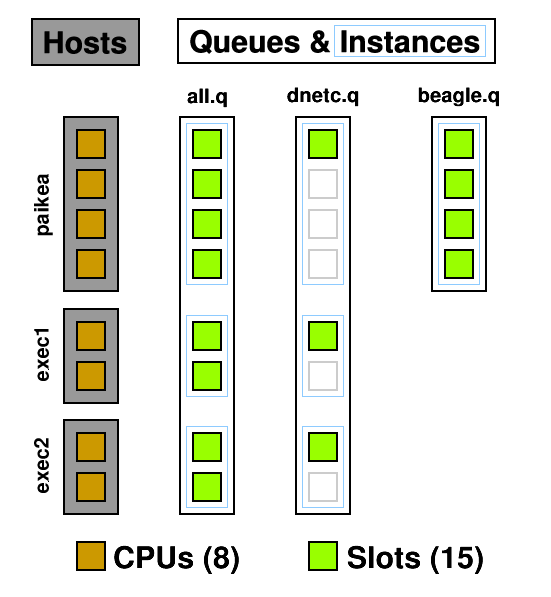
From this diagram you can see how CPUs can become oversubscribed. all.q covers every CPU. dnetc.q covers some of those CPUs a second time. Uh-oh! (dnetc.q is setup to use one slot per queue instance. That means that even if there are 10 CPUs on a given host, it will only use 1 of those.) This is something to consider when setting up queues and giving users access to them. Users can't put jobs into queues they don't have access to, so the only people causing contention are those with access to multiple queues but don't specify a queue ( -q ) when submitting.
Another use for queues are subordinate queues . I run low priority jobs in dnetc.q. When the main queue gets busy, all the jobs in dnetc.q are suspended until the main queue's load decreases. To do this I edited all.q, and under Subordinates added dnetc.q.
So far the shortest queue I've managed to make is one that uses 1 slot on each host it is allowed to run on. There is some talk in the documentation regarding user defined resources ( complexes ) which, much like licenses, can be "consumed" by jobs, thus limiting the number of concurrent jobs that can be run. (This may be useful for running an instance of Folding@Home, as it is not thread-safe , so you can set it up with a single "license".)
You can also change the default nice value of processes, but possibly the most useful setting is to turn on "rerunnable", which allows a task to be killed and run again on a different host.
Parallel Environment
Something that works better than queues and slots is to set up a
parallel environment. This can have a limited number of slots which counts over the entire grid and over every queue instance. As an example, Folding@Home is not thread safe. Each running thread needs its own work directory.How can you avoid contention in this case? Make each working directory a parallel environment, and limit the number of slots to 1.
I have four working directories named fah-a to fah-d . Each contains its own installation of the Folding@Home client:
$ ls ~/grid/fah-a/
fah-a
client.cfg
FAH504-Linux.exe
work
For each of these directories I have created a parallel environment:
admin@master:~$ qconf -sp fah-a
pe_name           fah-a
slots             1
user_lists        fah
These parallel environments are made available to all queues that the job can be run in and all users that have access to the working directory - which is just me.
The script to run the client is a marvel of grid arguments. It requests the parallel environment, bills the job to the Folding@Home project, names the project, etc. See for yourself:
#!/bin/sh
# use bash
#$ -S /bin/sh
# current directory
#$ -cwd
# merge output
#$ -j y
# mail at end
#$ -m e
# project
#$ -P fah
# name in queue
#$ -N fah-a
# parallel environment
#$ -pe fah-a 1
./FAH504-Linux.exe -oneunit
Note the -pe argument that says this job requires one slot worth of fah-a please.
Not a grid option, but the -oneunit flag for the folding client is important as this causes the job to quit after one work unit and the next work unit can be shuffled around to an appropriate host with a low load whose queue isn't disabled. Otherwise the client could end up running in a disabled queue for a month without nearing an end.
With the grid taking care of the parallel environment I no longer need to worry about manually setting up job holds so that I can enqueue multiple units for the same work directory. -t 1-20 ahoy!
Complex Configuration
An alternative to the parallel environment is to use a Complex. You create a new complex, say how many slots are available, and then let people consume them!
- In the QMON Complex Configuration, add a complex called "fah_l", type INT, relation <=, requestable YES, consumable YES, default 0. Add, then Commit.
- I can't manage to get this through QMON, so I do it from the command line. qconf -me global and then add fah_l=1 to the complex_values.
- Again through the command line. qconf -mq all.q and then add fah_l=1 to the complex_values. Change this value for the other queues. (Note that a value of 0 means jobs requesting this complex cannot be run in this queue.)
- When starting a job, add -l fah_l=1 to the requirements.
I had a problem to start off with, where qstat was telling me that -25 licenses were available. However this is due to the default value, so make sure that is 0!
Using Complexes I have set up license handling for Matlab and Splus .
- -l splus=1 (to request a Splus license)
- -l matlab=1 (to request a Matlab license)
- -l ml=1,matlabc=1 (to request a Matlab license and a Matlab Compiler license)
- -l ml=1,matlabst=1 (to request a Matlab license and a Matlab Statistics Toolbox license)
As one host group does not have Splus installed on them I simply set that host group to have 0 Splus licenses available. A license will never be available on the @gradroom host group, thus Splus jobs will never be queued there.
Quotas
Instead of Complexes and parallel environments, you could try a quota!
Please excuse the short details:
admin@master$ qconf -srqsl
admin@master$ qconf -mrqs lm2007_slots
{
   name         lm2007_slots
   description  Limit the lm2007 project to 20 slots across the grid
   enabled      TRUE
   limit        projects lm2007 to slots=20
}
Pending jobs
Want to know why a job isn't running?
- Job Control
- Pending Jobs
- Select a job
- Why ?
This is the same as qstat -f , shown at the bottom of this page.
Using Calendars
A calendar is a list of days and times along with states: off or suspended. Unless specified the state is on.
A queue, or even a single queue instance, can have a calendar attached to it. When the calendar says that the queue should now be "off" then the queue enters the disabled (D) state. Running jobs can continue, but no new jobs are started. If the calendar says it should be suspended then the queue enters the suspended (S) state and all currently running jobs are stopped (SIGSTOP).
First, create the calendar. We have an upgrade for paikea scheduled for 17 January:
admin@master$ qconf -scal paikeaupgrade
calendar_name    paikeaupgrade
year             17.1.2008=off
week             NONE
By the time we get around to opening up paikea's case and pull out the memory jobs will have had several hours to complete after the queue is disabled. Now, we have to apply this calendar to every queue instance on this host. You can do this all through qmon but I'm doing it from the command line because I can. Simply edit the calendar line to append the hostname and calendar name:
admin@master$ qconf -mq all.q
...
calendar              NONE,[paikea=paikeaupgrade]
...
Repeat this for all the queues.
There is a user who likes to use one particular machine and doesn't like jobs running while he's at the console. Looking at the usage graphs I've found out when he is using the machine and created a calendar based on this:
admin@master$ qconf -scal michael
calendar_name    michael
year             NONE
week             mon-sat=13-21=off
This calendar is obviously recurring weekly. As in the above example it was applied to queues on his machine. Note that the end time is 21, which covers the period from 2100 to 2159.
Suspending jobs automatically
Due to the number of slots being equal to the number of processors, system load is theoretically not going to exceed 1.00 (when divided by the number of processors). This value can be found in the np_load_* complexes .
But (and this is a big butt) there are a number of ways in which the load could go past a reasonable level:
- There are interactive users: all of the machines in the grad room (@gradroom) have console access.
- Someone logged in when they should not have: we're planning to disable ssh access to @ngaika except for %admins.
- A job is multi-threaded, and the submitter didn't mention this. If your Java program is using 'new Thread' somewhere, then it's likely you'll end up using multiple CPUs. Request more than one CPU when you're submitting the job. (-l slots=4 does not work.)
For example, with paikea , there are three queues:
- all.q (4 slots)
- paikea.q (4 slots)
- beagle.q (overlapping with the other two queues)
all.q is filled first, then paikea.q. beagle.q, by project and owner restrictions, is only available to the sponsor of the hardware. When their jobs come in, they can get put into beagle.q, even if the other slots are full. When the load average comes up, other tasks get suspended: first in paikea.q, then in all.q.
Let's see the configuration:
qname                 beagle.q
hostlist              paikea.stat.auckland.ac.nz
priority              19,[paikea.stat.auckland.ac.nz=15]
user_lists            beagle
projects              beagle
We have the limited access to this queue through both user lists and projects. Also, we're setting the Unix process priority to be higher than the other queues.
qname                 paikea.q
hostlist              paikea.stat.auckland.ac.nz
suspend_thresholds    NONE,[paikea.stat.auckland.ac.nz=np_load_short=1.01]
nsuspend              1
suspend_interval      00:05:00
slots                 0,[paikea.stat.auckland.ac.nz=4]
The magic here being that suspend_thresholds is set to 1.01 for np_load_short. This is checked every 5 minutes, and 1 process is suspended at a time. This value can be adjusted to get what you want, but it seems to be doing the trick according to graphs and monitoring the load. np_load_short is chosen because it updates the most frequently (every minute), more than np_load_medium (every five), and np_load_long (every fifteen minutes).
all.q is fairly unremarkable. It just defines four slots on paikea.
Submitting jobs Jobs are submitted to the Grid using qsub . Jobs are shell scripts containing commands to be run.
If you would normally run your job by typing ./runjob , you can submit it to the Grid and have it run by typing: qsub -cwd ./runjob
Jobs can be submitted while logged on to any submit host: sge-submit.stat.auckland.ac.nz .
For all the commands on this page I'm going to assume the settings are all loaded and you are logged in to a submit host. If you've logged in to a submit host then they'll have been sourced for you. You can source the settings yourself if required: . /opt/sge/default/common/settings.sh - the dot and space at the front are important .
Depending on the form your job is currently in they can be very easy to submit. I'm just going to go ahead and assume you have a shell script that runs the CPU-intensive computations you want and spits them out to the screen. For example, this tiny test.sh :
#!/bin/sh
expr 3 + 5
This computation is very CPU intensive!
Please note that the Sun Grid Engine ignores the bang path at the top of the script and will simply run the file using the queue's default shell which is csh. If you want bash, then request it by adding the very cryptic line: #$ -S /bin/sh
Now, let's submit it to the grid for running: Skip submission output
user@submit:~$ qsub test.sh
Your job 464 ("test.sh") has been submitted
user@submit:~$ qstat
job-ID  prior   name       user         state submit/start at     queue                slots ja-task-ID
-------------------------------------------------------------------------------------------------------
    464 0.00000 test.sh    user         qw    01/10/2008 10:48:03                          1
There goes our job, waiting in the queue to be run. We can run qstat a few more times to see it as it goes. It'll be run on some host somewhere, then disappear from the list once it is completed. You can find the output by looking in your home directory: Skip finding output
user@submit:~$ ls test.sh*
test.sh  test.sh.e464  test.sh.o464
user@submit:~$ cat test.sh.o464
8
The output file is named based on the name of the job, the letter o , and the number of the job.
If your job had problems running have a look in these files. They probably explain what went wrong.
Easiest way to submit R jobs
Here are two scripts and a symlink I created to make it easy as possible to submit R jobs to your Grid:
qsub-R
If you normally do something along the lines of:
user@exec:~$ nohup nice R CMD BATCH toodles.RNow all you need to do is:
user@submit:~$ qsub-R toodles.R
Your job 3540 ("toodles.R") has been submitted
qsub-R is linked to submit-R, a script I wrote. It calls qsub and submits a simple shell wrapper with the R file as an argument. It ends up in the queue and eventually your output arrives in the current directory: toodles.R.o3540
Download it and install it. You'll need to make the ' qsub-R ' symlink to ' 3rd_party/uoa-dos/submit-R ' yourself, although there is one in the package already for lx24-x86: qsub-R.tar (10 KiB, tar)
Thrashing the Grid
Sometimes you just want to give something a good thrashing, right? Never experienced that? Maybe it's just me. Anyway, here are two ideas for submitting lots and lots of jobs:
- Write a script that creates jobs and submits them
- Submit the same thing a thousand times
There are merits to each of these methods, and both of them mimic typical operation of the grid, so I'm going to explain them both.
Computing every permutation
If you have two lists of values and wish to calculate every permutation, then this method will do the trick. There's a more complicated solution below .
qsub will happily pass on arguments you supply to the script when it runs. Let us modify our test.sh to take advantage of this:
#!/bin/sh
#$ -S /bin/sh
echo Factors $1 and $2
expr $1 + $2
Now, we just need to submit every permutation to Grid:
user@submit:~$ for A in 1 2 3 4 5 ; do for B in 1 2 3 4 5 ; do qsub test.sh $A $B ; done ; doneAway the jobs go to be computed. If we have a look at different jobs we can see that it works. For example, job 487 comes up with:
user@submit:~$ cat test.sh.?487
Factors 3 and 5
8
Right on, brother! That's the same answer as we got previously when we hard coded the values of 3 and 5 into the file. We have algorithm correctness!
If we use qacct to look up the job information we find that it was computed on host mako (shark) and used 1 units of wallclock and 0 units of CPU.
Computing every permutation, with R
This method of creating job scripts and running them will allow you to compute every permutation of two variables. Note that you can supply arguments to your script, so it is not actually necessary to over-engineer your solution quite this much. This script has the added advantage of not clobbering previous computations. I wrote this solution for Yannan Jiang and Chris Wild and posted it to the r-downunder mailing list in December 2007. ( There is another method of doing this! )
In this particular example the output of the R command is deterministic, so it does not matter that a previous run (which could have taken days of computing time) gets overwritten, however I also work around this problem.
To start with I have my simple template of R commands (template.R):
alpha <- ALPHA
beta <- c(BETA)
# magic happens here
alpha
beta
The ALPHA and BETA parameters change for each time this simulation is run. I have these values stored, one per line, in the files ALPHA and BETA.
ALPHA:
0.9
0.8
0.7
BETA (please note that these contents must work both in filenames, bash commands, and R commands):
0,0,1
0,1,0
1,0,0
I have a shell script that takes each combination of ALPHA x BETA, creates a .R file based on the template, and submits the job to the Grid. This is called submit.sh:
#!/bin/sh

if [ "X${SGE_ROOT}" == "X" ] ; then
         echo Run: . /opt/sge/default/common/settings.sh
         exit
fi

cat ALPHA | while read ALPHA ; do
         cat BETA | while read BETA ; do
                 FILE="t-${ALPHA}-${BETA}"

                 # create our R file
                 cat template.R | sed -e "s/ALPHA/${ALPHA}/" -e "s/BETA/${BETA}/" > ${FILE}.R

                 # create a script
                 echo \#!/bin/sh > ${FILE}.sh
                 echo \#$ -S /bin/sh >> ${FILE}.sh
                 echo "if [ -f ${FILE}.Rout ] ; then echo ERROR: output file exists already ; exit 5 ; fi" >> ${FILE}.sh
                 echo R CMD BATCH ${FILE}.R ${FILE}.Rout >> ${FILE}.sh
                 chmod +x ${FILE}.sh

                 # submit job to grid
                 qsub -j y -cwd ${FILE}.sh
         done
done

qstat
When this script runs it will, for each permutation of ALPHA and BETA,
- create an R file based on the template, filling in the values of ALPHA and BETA,
- create a script that checks if this permutation has been calculated and then calls R,
- submits this job to the queue
... and finally shows the jobs waiting in the queue to execute.
Once computation is complete you will have a lot of files waiting in your directory. You will have:
- template.R -- our R commands template
- t-ALPHA-BETA.sh -- generated shell script that calls R
- t-ALPHA-BETA.R -- generated (from template) R commands
- t-ALPHA-BETA.Rout -- output from the command; this is a quirk of R
- t-ALPHA-BETA.sh.oNNN -- any output or errors from job (merged using qsub -j y )
The output files, stderr and stdout from when R was run, are always empty (unless something goes terribly wrong). For each permutation we receive four files. There are nine permutations (n ALPHA = 3, n BETA = 3, 3 × 3 = 9). A total of 36 files are created. (This example has been pared down from the original for purposes of demonstration.)
My initial question to the r-downunder list was how to get the output from R to stdout and thus t-ALPHA-BETA.sh.oNNN instead of t-ALPHA-BETA.Rout, however in this particular case, I have dodged that. In fact, being deterministic it is better that this job writes its output to a known filename, so I can do a one line test to see if the job has already been run.
I should also point out the -cwd option to the qsub command, which causes the job to be run in the current directory (which if it is in your home directory is accessible in the same place on all machines), rather than in /tmp/* . This allows us to find the R output, since R writes it to the directory it is currently in. Otherwise it could be discarded as a temporary file once the job ends!
Submit the same thing a thousand times
Say you have a job that, for example, pulls in random numbers and runs a simulation, or it grabs a work unit from a server, computes it, then quits. ( FAH -oneunit springs to mind, although it cannot be run in parallel. Refer to the parallel environment setup .) The script is identical every time.
SGE sets the SGE_JOB_ID environment variable which tells you the job number. You can use this as some sort of crude method for generating a unique file name for your output. However, the best way is to write everything to standard output (stdout) and let the Grid take care of returning it to you.
There are also Array Jobs which are
identical tasks being differentiated only by an index number, available through the -t option on qsub . This sets the environment variable of SGE_TASK_ID.For this example I will be using the Distributed Sleep Server . The Distributed Sleep Project passes out work units, packages of time, to clients who then process the unit. The Distributed Sleep Client, dsleepc , connects to the server to fetch a work unit. They can then be processed using the sleep command. A sample script: Skip sample script
#!/bin/sh
#$ -S /bin/sh
WORKUNIT=`dsleepc`
sleep $WORKUNIT && echo Processed $WORKUNIT seconds
Work units of 300 seconds typically take about five minutes to complete, but are known to be slower on Windows. (The more adventurous can add the -bigunit option to get a larger package for themselves, but note that they take longer to process.)
So, let us submit an array job to the Grid. We are going to submit one job with 100 tasks, and they will be numbered 1 to 100:
user@submit:~$ qsub -t 1-100 dsleep
Your job-array 490.1-100:1 ("dsleep") has been submitted
Job 490, tasks 1 to 100, are waiting to run. Later we can come back and pick up our output from our home directory. You can also visit the Distributed Sleep Project and check the statistics server to see if your work units have been received.
Note that running 100 jobs will fill the default queue, all.q. This has two effects. First, if you have any other queues that you can access jobs will be added to those queues and then run. (As the current setup of queues overlaps with CPUs this can lead to over subscription of processing resources. This can cause jobs to be paused, depending on how the queue is setup.) Second, any subordinate queues to all.q will be put on hold until the jobs get freed up.
Array jobs, with R
Using the above method of submitting multiple jobs, we can access this and use it in our R script, as follows: Skip R script
# alpha+1 is found in the SGE TASK number (qsub -t)
alphaenv <- Sys.getenv("SGE_TASK_ID")
alpha <- (as.numeric(alphaenv)-1)
Here the value of alpha is being pulled from the task number. Some manipulation is done of it, first to turn it from a string into a number, and secondly to change it into the expected form. Task numbers run from 1+, but in this case the code wants them to run from 0+.
Similar can be done with Java, by adding the environment value as an argument to invocation of the main class.
Advanced methods of queue submission
When you submit your job you have a lot of flexibility over it. Here are some options to consider that may make your life easier. Remember you can always look in the man page for qsub for more options and explanations.
qsub -N timmy test.shHere the job is called "timmy" and runs the script test.sh . Your the output files will be in timmy.[oe]*
The working directory is usually somewhere in /tmp on the execution host. To use a different working directory, eg, the current directory, use -cwd
qsub -cwd test.shTo request specific characteristics of the execution host, for example, sufficient memory, use the -l argument.
qsub -l mem_free=2500M test.shThis above example requests 2500 megabytes (M = 1024x1024, m = 1000x1000) of free physical memory (mem_free) on the remote host. This means it won't be run on a machine that has 2.0GB of memory, and will instead be put onto a machine with sufficient amounts of memory for BEAGLE Genetic Analysis . There are two other options for ensuring you get enough memory:
- Submit your job to the BEAGLE queue: -q beagle.q . This queue is specifically setup only on machines with a lot of free memory, and has 10 slots. You do have to be one of the allowed BEAGLE users to put jobs into this queue.
- Specify the amount of memory required in your script:
#$ -l mem=2500If your binary is architecture dependent you can ask for a particular architecture.
qsub -l arch=lx24-amd64 test.binThis can also be done in the script that calls the binary so you don't accidentally forget about including it.
#$ -l arch=lx24-amd64This requesting of resources can also be used to ask for a specific host, which goes against the idea of using the Grid to alleviate finding a host to use! Don't do this!
qsub -l hostname=mako test.shIf your job needs to be run multiple times then you can create an array job. You ask for a job to be run several times, and each run (or task) is given a unique task number which can be accessed through the environment variable SGE_TASK_ID. In each of these examples the script is run 50 times:
qsub -t 1-50 test.sh
qsub -t 75-125 test.sh
You can request a specific queue. Different queues have different characteristics.
- lm2007.q uses a maximum of one slot per host (although once I figure out how to configure it, it will use a maximum of six slots Grid-wide).
- dnetc.q is suspended when the main queue (all.q) is busy.
- beagle.q runs only on machines with enough memory to handle the data (although this can be requested with -l , as shown above).
qsub -q dnetc.q test.shA job can be held until a previous job completes. For example, this job will not run until job 380 completes:
qsub -hold_jid 380 test.shCan't figure out why your job isn't running? qstat can tell you:
qstat -j 490
... lots of output ...
scheduling info:            queue instance "[email protected]" dropped because it is temporarily not available
                            queue instance "[email protected]" dropped because it is full
                            cannot run in queue "all.q" because it is not contained in its hard queue list (-q)
Requesting licenses
Should you be using software that requires licenses then you should specify this when you submit the job. We have two licenses currently set up but can easily add more as requested:
- -l splus=1 (to request a Splus license)
- -l matlab=1 (to request a Matlab license)
- -l ml=1,matlabc=1 (to request a Matlab license and a Matlab Compiler license)
- -l ml=1,matlabst=1 (to request a Matlab license and a Matlab Statistics Toolbox license)
The Grid engine will hold your job until a Splus license or Matlab license becomes available.
Note: The Grid engine keeps track of the license pool independently of the license manager. If someone is using a license that the Grid doesn't know about, eg, an interactive session you left running on your desktop, then the count will be off. Believing a license is available, the Grid will run your job, but Splus will not run and your job will end. Here is a job script that will detect this error and then allow your job to be retried later: Skip Splus script
#!/bin/sh
#$ -S /bin/bash
# run in current directory, merge output
#$ -cwd -j y
# name the job
#$ -N Splus-lic
# require a single Splus license please
#$ -l splus=1
Splus -headless < $1
RETVAL=$?
if [ $RETVAL == 1 ] ; then
        echo No license for Splus
        sleep 60
        exit 99
fi
if [ $RETVAL == 127 ] ; then
        echo Splus not installed on this host
        # you could try something like this:
        #qalter -l splus=1,h=!`hostname` $JOB_ID
        sleep 60
        exit 99
fi
exit $RETVAL
Please note that the script exits with code 99 to tell the Grid to reschedule this job (or task) later. Note also that the script, upon receiving the error, sleeps for a minute before exiting, thus slowing the loop of errors as the Grid continually reschedules the job until it runs successfully. Alternatively you can exit with error 100, which will cause the job to be held in the error (E) state until manually cleared to run again.
You can clear a job's error state by using qmod -c jobid .
Here's the same thing for Matlab. Only minor differences from running Splus: Skip Matlab script
#!/bin/sh
#$ -S /bin/sh
# run in current directory, merge output
#$ -cwd -j y
# name the job
#$ -N ml
# require a single Matlab license please
#$ -l matlab=1

matlab -nodisplay < $1

RETVAL=$?
if [ $RETVAL == 1 ] ; then
        echo No license for Matlab
        sleep 60
        exit 99
fi
if [ $RETVAL == 127 ] ; then
        echo Matlab not installed on this host, `hostname`
        # you could try something like this:
        #qalter -l matlab=1,h=!`hostname` $JOB_ID
        sleep 60
        exit 99
fi
exit $RETVAL
Save this as "run-matlab". To run your matlab.m file, submit with: qsub run-matlab matlab.m
Processing partial parts of input files in Java
Here is some code I wrote for Lyndon Walker to process a partial dataset in Java.
It comes with two parts: a job script that passes the correct arguments to Java, and some Java code that extracts the correct information from the dataset for processing.
First, the job script gives some Grid task environment variables to Java. Our job script is merely translating from the Grid to the simulation:
java Simulation $@ $SGE_TASK_ID $SGE_TASK_LASTThis does assume your shell is bash, not csh. If your job is in 10 tasks, then SGE_TASK_ID will be a number between 1 and 10, and SGE_TASK_LAST will be 10. I'm also assuming that you are starting your jobs from 1, but you can also change that setting and examine SGE_TASK_FIRST.
Within Java we now read these variables and act upon them:
sge_task_id   = Integer.parseInt(args[args.length-2]);
sge_task_last = Integer.parseInt(args[args.length-1]);
For a more complete code listing, refer to sun-grid-qsub-java-partial.java (Simulation.java).
Preparing confidential datasets
The Grid setup here includes machines on which users can login. That creates the problem where someone might be able to snag a confidential dataset that is undergoing processing. One particular way to keep the files secure is as follows:
- Check we are able to securely delete files
- Locate a safe place to store files locally (the Grid sets up ${TMPDIR} to be unique for this job and task)
- Copy over dataset; it is expected you have setup password-less scp
- Preprocess dataset, eg, unencrypt
- Process dataset
- Delete dataset
A script that does this would look like the following: Skip dataset preparation script
#!/bin/sh
#$ -S /bin/sh

DATASET=confidential.csv

# check our environment
umask 0077
cd ${TMPDIR}
chmod 0700 .

# find srm
SRM=`which srm`
NOSRM=$?
if [ $NOSRM -eq 1 ] ; then
        echo system srm not found on this host, exiting >> /dev/stderr
        exit 99
fi

# copy files from data store
RETRIES=0
while [ ${RETRIES} -lt 5 ] ; do
        ((RETRIES++))
        scp user@filestore:/store/confidential/${DATASET} .
        if [ $? -eq 0 ] ; then
                RETRIES=5000
        else
                # wait for up to a minute (MaxStartups 10 by default)
                sleep `expr ${RANDOM} / 542`
        fi
done
if [ ! -f ${DATASET} ] ; then
        # unable to copy dataset after 5 retries, quit but retry later
        echo unable to copy dataset from store >> /dev/stderr
        exit 99
fi
# if you were decrypting the dataset, you would do that here

# copy our code over too
cp /mount/code/*.class .

# process data
java Simulation ${DATASET}

# collect results
# (We are just printing to the screen.)

# clean up
${SRM} -v ${DATASET} >> /dev/stderr

echo END >> /dev/stderr
Code will need to be adjusted to match your particular requirements, but the basic form is sketched out above.
As the confidential data is only in files and directories that root and the running user can access, and the same precaution is taken with the datastore, then only the system administrator and the user who has the dataset has access to these files.
The one problem here is how to manage the password-less scp securely. As this is run unattended, it would not be possible to have a password on a file, nor to forward authentication to some local agent. It may be possible to grab the packets that make up the key material. There must be a better way to do this. Remember that the job script is stored world-readable in the Grid cell's spool, so nothing secret can be put in there either.
Talk at Department Retreat
I gave a talk about the Sun Grid Engine on 19 February 2008-02-19 to the Department, giving a quick overview of the need for the grid and how to rearrange tasks to better make use of parallelism. It was aimed at end users and summarises into neat slides the reason for using the grid engine as well as a tutorial and example on how to use it all.
Download: Talk (with notes) PDF 5.9MiB
Question time afterwards was very good. Here are, as I recall them, the questions and answers.
Which jobs are better suited to parallelism?
Q (Ross Ihaka): Which jobs are better suited to parallelism? (Jobs with large data sets do not lend themselves to this sort of parallelism due to I/O overheads.)
A: Most of the jobs being used here are CPU intensive. The grid copies your script to /tmp on the local machine on which it runs. You could copy your data file across as well at the start of the job, thus all your later I/O is local.
(This is a bit of a poor answer. I wasn't really expecting it.) Bayesian priors and multiple identical simulations (eg, MCMC differing only by random numbers) lend themselves well to being parallelised.
Can I make sure I always run on the fastest machine?
A: The grid finds the machine with the least load to run jobs on. If you pile all jobs onto one host, then that host will slow down and become the slowest overall. Submit it through the grid and some days you'll get the fast host, and some days you'll get the slow host, and it is better in the long run. Also it is fair for other users. You can force it with -l, however, it is selfish.
Preemptable queues?
Q (Nicholas Horton): Is there support for preemptable queues? A person who paid for a certain machine might like it to be available only to them when they require it all for themselves.
A: Yes, the Grid has support for queues like that. It can all be configured. This particular example will have to be looked in to further. Beagle.q, as an example, only runs on paikea and overlaps with all.q . Also when the load on paikea , again using that as an example, gets too high, jobs in a certain queue (dnetc.q) are stopped.
An updated answer: the owner of a host can have an exclusive queue that preempts the other queues on the host. When the system load is too high, less important jobs can be suspended using suspend_thresholds .
Is my desktop an execution host?
Q (Ross Ihaka): Did I see my desktop listed earlier?
A: No. So far the grid is only running on the servers in the basement and the desktops in the grad room. Desktops in staff offices and used by PhD candidates will have to opt in.
(Ross Ihaka) Offering your desktop to run as an execution host increases the total speed of the grid, but your desktop may run slower at times. It is a two way street.
Is there job migration?
A: It's crude, and depends on your job. If something goes wrong (eg, the server crashes, power goes out) your job can be restarted on another host. When queue instances become unavailable (eg, we're upgrading paikea) they can send a signal to your job, telling it to save its work and quit, then can be restarted on another host.
Migration to faster hosts
Q (Chris Wild): What happens if a faster host becomes available while my job is running?
A: Nothing. Your job will continue running on the host it is on until it ends. If a host is overloaded, and not due to the grid's fault, some jobs can be suspended until load decreases . The grid isn't migrating jobs. The best method is to break your job down into smaller jobs, so that when the next part of the job is started it gets put onto what is currently the best available host.
Over sufficient jobs it will become apparent that the faster host is processing more jobs than a slower host.
Desktops and calendars
Q (Stephane Guindon): What about when I'm not at my desktop. Can I have my machine be on the grid then, and when I get to the desktop the jobs are migrated?
A: Yes, we can set up calendars so that at certain times no new jobs will be started on your machine. Jobs that are already running will continue until they end. (Disabling the queue.) Since some jobs run for days this can appear to have no influence on how many jobs are running. Alternatively jobs can be paused, which frees up the CPU, but leaves the job sitting almost in limbo. (Suspending the queue.) Remember the grid isn't doing migration. It can stop your job and run it elsewhere (if you're using the -notify option on submission and handling the USR1 signal).
Jobs under the grid
Q (Sharon Browning): How can I tell if a job is running under the grid's control? It doesn't show this under top .
A: Try ps auxf . You will see the job taking a lot of CPU time, the parent script, and above that the grid (sge_shepherd and sge_execd).
Talk for Department Seminar
On September 11 I gave a talk to the Department covering:
- Trends in Supercomputing
- Increase in power
- Increase in power consumption
- Increase in data
- Collection of servers
- Workflows
- Published services
- Collaboration
- How to use it
- Jargon
- Taking advantage of more CPUs
- Rewriting your code
- Case Studies
- Increasing your Jargon
- Question time
Download slides with extensive notes: Supercomputing and You (PDF 3MiB)
A range of good questions:
- What about psuedo-random number generators being initialised with the same seed?
- How do I get access to these resources if I'm not a researcher here?
- How do I get access to this Department's resources?
- Do Windows programs (eg, WinBUGS) run on the Grid?
Summary
In summary, I heartily recommend the Sun Grid Engine. After a few days installation, configuring, messing around, I am very impressed with what can be done with it.
Try it today.
Aug 17, 2018 | www.rocksclusters.org
Operating System Base
Rocks 7.0 (Manzanita) x86_64 is based upon CentOS 7.4 with all updates available as of 1 Dec 2017.
Building a bare-bones compute clusterBuilding a more complex cluster
- Boot your frontend with the kernel roll
- Then choose the following rolls: base , core , kernel , CentOS and Updates-CentOS
In addition to above, select the following rolls:
Building Custom Clusters
- area51
- fingerprint
- ganglia
- kvm (used for virtualization)
- hpc
- htcondor (used independently or in conjunction with sge)
- perl
- python
- sge
- zfs-linux (used to build reliable storage systems)
If you wish to build a custom cluster, you must choose from our a la carte selection, but make sure to download the required base , kernel and both CentOS rolls. The CentOS rolls include CentOS 7.4 w/updates pre-applied. Most users will want the full updated OS so that other software can be added.
MD5 ChecksumsPlease double check the MD5 checksums for all the rolls you download.
DownloadsAll ISOs are available for downloads from here . Individual links are listed below.
Name Description Name Description kernel Rocks Bootable Kernel Roll required zfs-linux ZFS On Linux Roll. Build and Manage Multi Terabyte File Systems. base Rocks Base Roll required fingerprint Fingerprint application dependencies core Core Roll required hpc Rocks HPC Roll CentOS CentOS Roll required htcondor HTCondor High Throughput Computing (version 8.2.8) Updates-CentOS CentOS Updates Roll required sge Sun Grid Engine (Open Grid Scheduler) job queueing system kvm Support for building KVM VMs on cluster nodes perl Support for Newer Version of Perl ganglia Cluster monitoring system from UCB python Python 2.7 and Python 3.x area51 System security related services and utilities openvswitch Rocks integration of OpenVswitch
Oct 15, 2017 | biohpc.blogspot.com
Installation of Son of Grid Engine(SGE) on CentOS7
SGE Master installation
master# hostnamectl set-hostname qmaster.local
master# vi /etc/hosts
192.168.56.101 qmaster.local qmaster
192.168.56.102 compute01.local compute01master# mkdir -p /BiO/src
master# yum -y install epel-release
master# yum -y install jemalloc-devel openssl-devel ncurses-devel pam-devel libXmu-devel hwloc-devel hwloc hwloc-libs java-devel javacc ant-junit libdb-devel motif-devel csh ksh xterm db4-utils perl-XML-Simple perl-Env xorg-x11-fonts-ISO8859-1-100dpi xorg-x11-fonts-ISO8859-1-75dpi
master# groupadd -g 490 sgeadmin
master# useradd -u 495 -g 490 -r -m -d /home/sgeadmin -s /bin/bash -c "SGE Admin" sgeadmin
master# visudo
%sgeadmin ALL=(ALL) NOPASSWD: ALL
master# cd /BiO/src
master# wget http://arc.liv.ac.uk/downloads/SGE/releases/8.1.9/sge-8.1.9.tar.gz
master# tar zxvfp sge-8.1.9.tar.gz
master# cd sge-8.1.9/source/
master# sh scripts/bootstrap.sh && ./aimk && ./aimk -man
master# export SGE_ROOT=/BiO/gridengine && mkdir $SGE_ROOT
master# echo Y | ./scripts/distinst -local -allall -libs -noexit
master# chown -R sgeadmin.sgeadmin /BiO/gridenginemaster# cd $SGE_ROOT
master# ./install_qmaster
press enter at the intro screen
press "y" and then specify sgeadmin as the user id
leave the install dir as /BiO/gridengine
You will now be asked about port configuration for the master, normally you would choose the default (2) which uses the /etc/services file
accept the sge_qmaster info
You will now be asked about port configuration for the master, normally you would choose the default (2) which uses the /etc/services file
accept the sge_execd info
leave the cell name as "default"
Enter an appropriate cluster name when requested
leave the spool dir as is
press "n" for no windows hosts!
press "y" (permissions are set correctly)
press "y" for all hosts in one domain
If you have Java available on your Qmaster and wish to use SGE Inspect or SDM then enable the JMX MBean server and provide the requested information - probably answer "n" at this point!
press enter to accept the directory creation notification
enter "classic" for classic spooling (berkeleydb may be more appropriate for large clusters)
press enter to accept the next notice
enter "20000-20100" as the GID range (increase this range if you have execution nodes capable of running more than 100 concurrent jobs)
accept the default spool dir or specify a different folder (for example if you wish to use a shared or local folder outside of SGE_ROOT
enter an email address that will be sent problem reports
press "n" to refuse to change the parameters you have just configured
press enter to accept the next notice
press "y" to install the startup scripts
press enter twice to confirm the following messages
press "n" for a file with a list of hosts
enter the names of your hosts who will be able to administer and submit jobs (enter alone to finish adding hosts)
skip shadow hosts for now (press "n")
choose "1" for normal configuration and agree with "y"
press enter to accept the next message and "n" to refuse to see the previous screen again and then finally enter to exit the installermaster# cp /BiO/gridengine/default/common/settings.sh /etc/profile.d/
master# qconf -ah compute01.local
compute01.local added to administrative host listmaster# yum -y install nfs-utils
master# vi /etc/exports
/BiO 192.168.56.0/24(rw,no_root_squash)master# systemctl start rpcbind nfs-server
master# systemctl enable rpcbind nfs-serverSGE Client installation
compute01# yum -y install hwloc-devel
compute01# hostnamectl set-hostname compute01.local
compute01# vi /etc/hosts
192.168.56.101 qmaster.local qmaster
192.168.56.102 compute01.local compute01compute01# groupadd -g 490 sgeadmin
compute01# useradd -u 495 -g 490 -r -m -d /home/sgeadmin -s /bin/bash -c "SGE Admin" sgeadmincompute01# yum -y install nfs-utils
compute01# systemctl start rpcbind
compute01# systemctl enable rpcbind
compute01# mkdir /BiO
compute01# mount -t nfs 192.168.56.101:/BiO /BiO
compute01# vi /etc/fstab
192.168.56.101:/BiO /BiO nfs defaults 0 0compute01# export SGE_ROOT=/BiO/gridengine
compute01# export SGE_CELL=default
compute01# cd $SGE_ROOT
compute01# ./install_execd
compute01# cp /BiO/gridengine/default/common/settings.sh /etc/profile.d/
Jun 21, 2018 | community.pbspro.org
How to install pbs on compute node and configure the server and compute node? Users/Site Administrators You have selected 0 posts.
cancel selecting Jun 2016 1 / 9 Jul 2016 Apr 2017 Joey Jun '16 Hi guys,
I am new to HPC and PBS or torque. I am able to install PBS pro from source code on my head node . But not sure how to install the compute node and cconfigure it. I didn't see any documentation in the github either. Can anyone give me some help? Thanksbuchmann Jun '16 Install is pretty similar on the compute nodes - however, you do not need the "server" parts.
There are OK docs on the Altair "pro" site, see answer to previous question "documentation-is-missing/81".In short, you the Altair docs for v13, and/or the INSTALL file procedure. (Or install from pre-build binaries).
Actual method will depend on your system type etc.I prefer to install using pre-compiled RPMs (CentOS72 systems), which presently means that I will compile these from tarball+spec-file (slightly modified spec-file).
Hope this helps.
/Bjarne subhasisb Jun '16 @Joey thanks for joining the pbspro forum.You can find the documentation about pbspro here: https://pbspro.atlassian.net/wiki/display/PBSPro/User+Documentation 730
Kindly do not hesitate to post questions about any specific issues you are facing.
Thanks,
Subhasis Joey Jun '16 1 Thanks for your reply.I rebuild the CentOS72 rpm with the src from Centos7.zip
installed pbspro-server-14.1.0-13.1.x86_64.rpm on mye headnode
installed pbspro-execution-14.1.0-13.1.x86_64.rpm on my compute node.
On the head node
create /var/spool/pbs/server_priv/nodes with following:computenode1 np=1
/etc/pbs.conf:
PBS_SERVER=headnode
PBS_START_SERVER=1
PBS_START_SCHED=1
PBS_START_COMM=1
PBS_START_MOM=0
PBS_EXEC=/opt/pbs
PBS_HOME=/var/spool/pbs
PBS_CORE_LIMIT=unlimited
PBS_SCP=/bin/scpon the compute node
/var/spool/pbs/mom_priv/config as following
$logevent 0x1ff
$clienthost headnode
$restrict_user_maxsysid 999/etc/pbs.conf
PBS_SERVER=headnode
PBS_START_SERVER=0
PBS_START_SCHED=0
PBS_START_COMM=0
PBS_START_MOM=1
PBS_EXEC=/opt/pbs
PBS_HOME=/var/spool/pbs
PBS_CORE_LIMIT=unlimited
PBS_SCP=/bin/scpafter that I start the pbs on headnode and compute node without error:
#/etc/init.d/pbs start
But when I try to run pbsnodes -a, it tells me:
pbsnodes: Server has no node list
If I run a script it will just Queue there.Both server firewalld are turned off and pingable.
Can anyone give me some help? Thanks subhasisb Jul '16 Hi @Joey ,
Unlike torque, pbspro uses a real relational database underneath to store information about nodes, queues, jobs etc. Thus creating a nodes file is not supported under pbspro.
To add a node to pbs cluster, use the qmgr command as follows:
qmgr -c "create node hostname"
HTH
regards,
Subhasis Joey Jul '16 Thanks for your reply. I thought PBS and torque are the same except one is open source and one is commerical. subhasisb Jul '16 Hi @JoeyThey might feel similar since Torque was based on the OpenPBS codebase. OpenPBS was a version of PBS released as opensource many years back.
Post that, Altair engineering has put in a huge amount of effort towards PBS Professional and added tons of features and improvements in terms of scalability, robustness and ease of use over decades which resulted in it becoming the number one work load manager in the HPC world. Altair has now open-sourced PBS Professional.
So, pbspro is actually very different from torque in terms of capability and performance, and is actually a completely different product.
Let us know if you need further information in switching to pbspro.
Thanks and Regards,
Subhasis 10 months later sxy Apr '17 Hi Subhasis,To add a node to pbs cluster, use the qmgr command as follows:
qmgr -c "create node hostname"
if a site has a few hundreds of compute nodes, the above method is very tedious.
would there be any easy/quick ways to register computer nodes with pbs server like the nodes file in torque?Thanks,
Sue mkaro Apr '17 This is one way to accomplish it
while read line; do [ -n "$line" ] && qmgr -c "create node $line"; done <nodefilewhere nodefile contains the list of nodes, one per line.
Jun 13, 2018 | www.admin-magazine.com
The King in Alice in Wonderland said it best, "Begin at the beginning ." The general goal of HPC is either to run applications faster or to run problems that can't or won't run on a single server. To do this, you need to run parallel applications across separate nodes. Although you could use a single node and then create two VMs, it's important to understand how applications run across physically different servers and how you administer a system of disparate physical hardware.
With this goal in mind, you can make some reasonable assumptions about the HPC system. If you are interested in parallel computing using multiple nodes, you need at least two separate systems (nodes), each with its own operating system (OS). To keep things running smoothly, the OS on both nodes should be identical. (Strictly speaking, it doesn't have to be this way, but otherwise, it is very difficult to run and maintain.) If you install a package on node 1, then it needs to be installed on node 2 as well. This lessens a source of possible problems when you have to debug the system.
The second thing your cluster needs is a network to connect the nodes so they can communicate to share data, the state of the solution to the problem, and possibly even the instructions that need to be executed. The network can theoretically be anything that allows communication between nodes, but the easiest solution is Ethernet. In this article, I am initially going to consider a single network, but later I will consider more than one.
Storage in each node can be as simple as an SD card to hold the OS, the applications, and the data. In addition to some basic storage, and to make things a bit easier, I'll create a shared filesystem from the master node to the other nodes in the cluster.
The most fundamental HPC architecture and software is pretty unassuming. Most distributions have the basic tools for making a cluster work and for administering the tools; however, you will most likely have to add the tools and libraries for the parallel applications (e.g., a message-passing interface [MPI] library or libraries, compilers, and any additional libraries needed by the application). Perhaps surprisingly, the other basic tools are almost always installed by default on an OS; however, before discussing the software, you need to understand the architecture of a cluster.
Architecture
The architecture of a cluster is pretty straightforward. You have some servers (nodes) that serve various roles in a cluster and that are connected by some sort of network. That's all. It's that simple. Typically the nodes are as similar as possible, but they don't have to be; however, I highly recommend that they be as similar as possible because it will make your life much easier. Figure 1 is a simple illustration of the basic architecture.
Figure 1: Generic cluster layout.
Almost always you have a node that serves the role of a "master node" (sometimes also called a "head node"). The master node is the "controller" node or "management" node for the cluster. It controls and performs the housekeeping for the cluster and many times is the login node for users to run applications. For smaller clusters, the master node can be used for computation as well as management, but as the cluster grows larger, the master node becomes specialized and is not used for computation.
Other nodes in the cluster fill the role of compute nodes, which describes their function. Typically compute nodes don't do any cluster management functions; they just compute. Compute nodes are usually systems that run the bare minimum OS – meaning that unneeded daemons are turned off and unneeded packages are not installed – and have the bare minimum hardware.
As the cluster grows, other roles typically arise, requiring that nodes be added. For example, data servers can be added to the cluster. These nodes don't run applications; rather, they store and serve data to the rest of the cluster. Additional nodes can provide data visualization capabilities within the cluster (usually remote visualization), or very large clusters might need nodes dedicated to monitoring the cluster or to logging in users to the cluster and running applications.
For a simple two-node cluster that you might use as your introduction to HPC, you would typically designate one master node and one compute node. However, because you only have two nodes, applications would most likely run on both – because why waste 50% of your nodes?
The network connecting the cluster nodes could be any networking technology, but the place to start is with wired Ethernet, which ranges from 100Mbps to 56Gbps; however, I'll stick to the more common Fast Ethernet (100Mbps) or Gigabit Ethernet (1,000Mbps).
The network topology you use for clusters is important because it can have an effect on application performance. If you are just starting out, I would stick to the basics. A simple network layout has a single switch with all nodes plugged in to that switch. This setup, called a fat tree topology , has only one level and is simple and effective, particularly when building smaller systems. As systems get larger, you can still stick to the fat tree topology, but you will likely have to have more levels of switches. If you re-use your existing switches, design the topology carefully so you don't introduce bottlenecks.
For smaller systems, Ethernet switches are pretty inexpensive, costing just a few dollars per port. Switches are going to be better than an Ethernet hub, but if all you have is a hub, then you can use it. Although hubs will limit performance, it won't stop the cluster from working.
Because you're interested in "high performance," you want to do everything possible to keep the cluster network from reducing performance. A common approach is to put the cluster on a private Ethernet network. The address space is unroutable, so the compute nodes will effectively be "hidden" from a routable network, allowing you to separate your cluster logically from a public network.
However, a good idea would be to log in to the cluster from a public network, and the way to do that when the cluster is on a private network is to add a second network interface controller (NIC) to the master node. This NIC will have a public IP address that allows you to log in to the cluster. Only the master node should have the public IP address, because there is no reason for compute nodes to have two addresses. (You want them to be private.) For example, you can make the public address for the master node something like 72.x.x.x and the private address something like 10.x.x.x. The order of the network interfaces doesn't make a huge difference, but you have to pay attention to them when installing the OS.
You can give the master node two private addresses if you are behind a network address translator (NAT). This configuration is very common in home routers, which are also NAT devices. For example, in my home network, I have an Internet router that is really a NAT. It converts packets from a private network, such as 192.168.x.x, to the address of the router (the Internet) and vice versa. My simple clusters have a master node with a public IP of 192.168.x.x, and they have a second NIC with an address of 10.x.x.x, which is the cluster's private network.
Another key feature of a basic cluster architecture is a shared directory across the nodes. Strictly speaking this isn't required, but without it, some MPI applications would not run. Therefore, it is a good idea simply to use a shared filesystem in the cluster. NFS is the easiest to use because both server and client are in the kernel, and the distribution should have the tools for configuring and monitoring NFS.
The classic NFS approach to a shared directory is to export a directory from the master node to the compute nodes. You can pick any directory you want to export, but many times, people just share /home from the master node, although sometimes they will also export a new directory, such as /shared . The compute nodes also mount the shared directory as /home . Therfore, if anything in /home is local to each node, it won't be accessible.
Of course, you can get much fancier and more complicated, and you might have good reasons to do so, but in general you should adopt the KISS (Keep It Simple Silly) approach. Simple means it is easier to debug problems. Simple also means it's easier to reconfigure the cluster if you want (or need). With the architecture established, I'll turn to the software you'll need.
Software Layers
Unfortunately, no single secret magic pixie dust can be sprinkled on a cluster to make it work magically and run applications in parallel. It takes careful thought and planning to operate a set of separate systems as a single system. This is especially true for the cluster software.
This article is really about the basics of HPC, so I want to start with the basic software you need to run parallel applications. However, additional tools can be added to make operating the cluster much easier for the administrator, as well as tools to make life easier for people using the cluster. Rather than just provided yet another list of these tools, I want to present them in three layers. The first layer is the basic software you need and really nothing extra. The second layer adds some administrative tools to make it easier to operate the cluster, as well as tools to reduce problems when running parallel applications. The third layer adds more sophisticated cluster tools and adds the concept of monitoring, so you can understand what's happening.
Layer 1: Software Configuration
The first layer of software only contains the minimum software to run parallel applications. Obviously, the first thing you need is an OS. Typical installation options are usually good enough. They install most everything you need.
The next thing you need is a set of MPI libraries such as Open MPI or MPICH . These are the libraries you will use for creating parallel applications and running them on your cluster. You can find details on how to build and install them on their respective websites.
Each node has to have the same libraries for the MPI applications to run. You have two choices at this point: build, install, and set up the appropriate paths for the libraries in your shared directory or build and install the libraries on each node individually. The easiest choice is to install the source packages in the shared directory.
The next, and actually last, piece of software you need is SSH. More specifically, you need to be able to SSH to and from each node without a password, allowing you to run the MPI applications easily. Make sure, however, that you set up SSH after you have NFS working across the cluster and each node has mounted the exported directory.
In addition to NFS across the cluster, you need the same users and groups on the nodes. Because you have to create the same user on every node (recall that the OS is specific to each node), this can be a monumental pain if you have a few thousand nodes.
Running applications with this configuration is not too difficult because the nodes have a shared directory. Note also that you can have more than one shared directory. I'll assume that you will compile your MPI application on your master node in your home directory (e.g., / home/laytonjb/bin/<app> , where <app> is the executable. The directory /home , can be shared across the cluster so that each node can access the application and the same input and output files (presumably the input and output files are in the shared directory).
As the application starts, SSH is used to communicate between MPI ranks (the MPI processes). Because you can SSH without using passwords, the application should run without problems. The details of running your MPI application depends on your MPI library, which typically provides a simple script or small executable to run the application.
This software configuration is the bare minimum to allow you to run applications. Even then you might have some issues, but with some careful consideration you should be able to run applications.
Layer 2: Architecture and Tools
The next layer of software adds tools to help reduce cluster problems and make it easier to administer. Using the basic software mentioned in the previous section, you can run parallel applications, but you might run into difficulties as you scale your system, including:
- Running commands on each node (parallel shell)
- Configuring identical nodes (package skew)
- Keeping the same time on each node (NTP)
- Running more than one job (job scheduler/resource manager)
These issues arise as you scale the cluster, but even for a small two-node cluster, they can become problems.
First, you need to be able to run the same command on every node, so you don't have to SSH to each and every node. One solution would be to write a simple shell script that takes the command line arguments as the "command" and then runs the command on each node using SSH. However, what happens if you only want to run the command on a subset of the nodes? What you really need is something called a parallel shell.
A number of parallel shell tools are available, and the most common is pdsh , which lets you run the same command across each node. However, simply having a parallel shell doesn't mean the cluster will magically solve all problems, so you have to develop some procedures and processes. More specifically, you can use a parallel shell to overcome the second issue: package skew.
Package skew can cause lots of problems for HPC admins. If you have an application that runs fine one day, but try it again the next day and it won't run, you have to start looking for reasons why. Perhaps during the 24-hour period, a node that had been down suddenly comes back to life, and you start running applications on it. That node might not have the same packages or the same versions of software as the other nodes. As a result, applications can fail, and they can fail in weird ways. Using a parallel shell, you can check that each node has the package installed and that the versions match.
To help with package skew, I recommend after first building the cluster and installing a parallel shell you start examining key components of the installation. For example, check the following:
- glibc version
- GCC version
- GFortran version
- SSH version
- Kernel version
- IP address
- MPI libraries
- NIC MTU – Use ifconfig
- BogoMips – Although this number is meaningless, it should be the same across nodes if you are using the same hardware. To check this number, enter:
cat /proc/cpuinfo | grep bogomips
- Nodes have the same amount of memory (if they are identical):
cat /proc/meminfo | grep MemTotalMany more package versions or system information can be checked, which you can store in a spreadsheet for future reference. The point is that doing this at the very beginning and then developing a process or procedure for periodically checking the information is important. You can quickly find package skew problems as they occur and correct them.
I also recommend keeping a good log so that if a node is down when you install or update packages, you can come back to it when the node is back up. Otherwise, you start getting package skew in your nodes and subsequent problems.
The third issue to overcome is keeping the same time on each node. The Network Time Protocol synchronizes system clocks. Most distributions install ntp by default and enable it, but be sure you check for it in each node in the cluster – and check the version of ntpd as well.
Use chkconfig , if the distribution has this package, to check that ntp is running. Otherwise, you will have to look at the processes running on the nodes to see whether ntpd is listed (hint – use your parallel shell). Configuring NTP can be a little tricky, because you have to pay attention to the architecture of the cluster.
On the master node, make sure that the NTP configuration file points to external servers (outside the cluster) and that the master node can resolve these URLs (try using either ping to ping each server or nslookup ). Also be sure the ntpd daemon is running.
For nodes that are on a private network that doesn't have access to the Internet, you should configure NTP to use the master node as the timekeeper. This can be done by editing /etc/ntp.conf and changing the NTP servers to point to the master node's IP address. Roughly, it should look something like Listing 1. The IP address of the master node is 10.1.0.250. Be sure to check that the compute nodes can ping this address. Also be sure that ntp starts when the nodes are booted.
[root@test1 etc]# more ntp.conf
# For more information about this file, see the man pages
# ntp.conf(5), ntp_acc(5), ntp_auth(5), ntp_clock(5), ntp_misc(5), ntp_mon(5).

#driftfile /var/lib/ntp/drift

restrict default ignore
restrict 127.0.0.1
server 10.1.0.250
restrict 10.1.0.250 nomodify
The last issue to address is the job scheduler (also called a resource manager). This is a key element of HPC and can be used even for small clusters. Roughly speaking, a job scheduler will run jobs (applications) on your behalf when the resources are available on the cluster, so you don't have to sit around and wait for the cluster to be free before you run applications. Rather, you can write a few lines of script and submit it to the job scheduler. When the resources are available, it will run your job on your behalf. (Resource managers allow HPC researchers to actually get some sleep.)
In the script, you specify the resources you need, such as the number of nodes or number of cores, and you give the job scheduler the command that runs your application, such as:
mpirun -np 4 <executable>Among the resource managers available, many are open source, and they usually aren't too difficult to install and configure; however, be sure you read the installation guide closely. Examples of resource managers include:
With these issues addressed, you now have a pretty reasonable cluster with some administrative tools. Although it's not perfect, it's most definitely workable. However, you can go to another level of tools, which I refer to as the third layer, to really make your HPC cluster sing.
Layer 3: Deep Administration
The third level of tools gets you deeper into HPC administration and begins to gather more information about the cluster, so you can find problems before they happen. The tools I will discuss briefly are:
- Cluster management tools
- Monitoring tools (how are the nodes doing)
- Environment Modules
- Multiple networks
A cluster management tool is really a toolkit to automate the configuration, launching, and management of compute nodes from the master node (or a node designated a master). In some cases, the toolkit will even install the master node for you. A number of open source cluster management tools are available, including:
Some very nice commercial tools exist as well.
The tools vary in their approach, but they typically allow you to create compute nodes that are part of the cluster. This can be done via images, in which a complete image is pushed to the compute node, or via packages, in which specific packages are installed on the compute nodes. How this is accomplished varies from tool to tool, so be sure you read about them before installing them.
The coolest thing about these tools is that they remove the drudgery of installing and managing compute nodes. Even with four-node clusters, you don't have to log in to each node and fiddle with it. The ability to run a single command and re-install identical compute nodes can eliminate so many problems when managing your cluster.
Many of the cluster management tools also include tools for monitoring the cluster. For example, being able to tell which compute nodes are up or down or which compute nodes are using a great deal of CPU (and which aren't) is important information for HPC administrators. Monitoring the various aspects of your nodes, including gathering statistics on the utilization of your cluster can be used when it's time to ask the funding authorities for additional hardware, whether it be the household CFO, a university, or an agency such as the National Science Foundation. Regardless of who it is, they will want to see statistics about how heavily the cluster is being used.
Several monitoring tools are appropriate for HPC clusters, but a universal tool is Ganglia . Some of the cluster tools come pre-configured with Ganglia, and some don't, requiring an installation . By default Ganglia comes with some pre-defined metrics, but the tool is very flexible and allows you to write simple code to attain specific metrics from your nodes.
Up to this point, you have the same development tools, the same compilers, the same MPI libraries, and the same application libraries installed on all of your nodes. However, what if you want to install and use a different MPI library? Or what if you want to try a different version of a particular library? At this moment you would have to stop all jobs on the cluster, install the libraries or tools you want, make sure they are in the default path, and then start the jobs again. This process sounds like an accident waiting to happen. The preventive is called environment modules.
Originally, environment modules were developed to address the problem of having applications that need different libraries or compilers by allowing you to modify your user environment dynamically with module files. You can load a module file that specifies a specific MPI library or makes a specific compiler version the default. After you build your application using these tools and libraries, if you run an application that uses a different set of tools, you can "unload" the first module file and load a new module file that specifies a new set of tools. It's all very easy to do with a job script and is extraordinarily helpful on multiuser systems.
Lmod is a somewhat new version of environment modules that addresses the need for module hierarchies (in essence, module dependencies) so that a single module "load" command can load a whole series of modules. Lmod currently is under very active development.
Up to now I have assumed that all traffic in the cluster, including administration, storage, and computation, use the same network. For improved computational performance or improved storage performance, though, you might want to contemplate separating the traffic into specific networks. For example, you might consider a separate network just for administration and storage traffic, so that each node has two private networks: one for computation and one for administration and storage. In this case, the master node might have three network interfaces.
Separating the traffic is pretty easy by giving each network interface (NIC) in the node an IP address with a different address range. For example, eth0 might be on a 10.0.1.x network, and eth1 on 10.0.2.x network. Although theoretically you could give all interfaces an address in the same IP range, different IP ranges just make administration easier. Now when you run MPI applications, you use addresses in 10.0.1.x. For NFS and any administration traffic, you would use addresses in 10.0.2.x. In this way, you isolate computational traffic from all other traffic.
The upside to isolating traffic is additional bandwidth in the networks. The downside is twice as many ports, twice as many cables, and a little more cost. However, if the cost and complexity isn't great, using two networks while you are learning cluster administration, or even writing applications, is recommended.
Summary
Stepping back to review the basics is a valuable exercise. In this article I wanted to illustrate how someone could get started creating their own HPC system. If you have any comments, post to the Beowulf mailing list . I'll be there, as will a number of other people who can help.
Apr 25, 2018 | github.com
nicoulaj commented
on Dec 1 2016 FYI, I got a working version with SGE on CentOS 7 on my linked branch.
This is quick and dirty because I need it working right now, there are several issues:
- I inverted the SGE setup/NFS export order due to #347 , so Debian support is probably broken
- The RPMs for RHEL do not contain systemd init files, so there are some workarounds to start
sge_execdmanually- I used
set_factto set global variables forSGE_ROOT, maybe there is a cleaner way ? I never used Ansible until now, I don't know the good practices...
Apr 24, 2018 | liv.ac.uk
From: JuanEsteban.Jimenez at mdc-berlin.de [mailto: JuanEsteban.Jimenez at mdc-berlin.de ]
Sent: 27 April 2017 03:54 PM
To: yasir at orionsolutions.co.in ; 'Maximilian Friedersdorff'; sge-discuss at liverpool.ac.uk
Subject: Re: [SGE-discuss] SGE Installation on Centos 7I am running SGE on nodes with both 7.1 and 7.3. Works fine on both.
Just make sure that if you are using Active Directory/Kerberos for authentication and authorization, your DC's are capable of handling a lot of traffic/requests. If not, things like DRMAA will uncover any shortcomings.
Mfg,
Juan Jimenez
System Administrator, BIH HPC Cluster
MDC Berlin / IT-Dept.
Tel.: +49 30 9406 2800====================
I installed SGE on Centos 7 back in January this year. If my recolection is correct, the procedure was analogous to the instructions for Centos 6. There were some issues with the firewalld service (make sure that it is not blocking SGE), as well as some issues with SSL.
Check out these threads for reference:http://arc.liv.ac.uk/pipermail/sge-discuss/2017-January/001047.html
http://arc.liv.ac.uk/pipermail/sge-discuss/2017-January/001050.html
Apr 20, 2018 | lists.sdsc.edu
[Rocks-Discuss] Environment Modules Recommendations
>> 1. I use the C modules code. But, I like the tcl version better. It seems more robust and it is certainly easier to fix (or not -- like the erroneous "Duplicate version symbol" below) and enhance (as I have done). I think I'll switch the next time I upgrade our cluster.
>> 2. I have come to not like the recommended organizational scheme of package/version. I think I'll switch to using the version as a suffix, like RPMs do, e.g. package-version. I think that would make it easier to use the built-in default selection mechanism (alphabetic ordering, last one is the default). Right now, for example, my modules are:
Environment Modules - Mailing Lists
[Modules] Duplicate version symbol found
[Modules] Duplicate version symbol found From: Christoph Niethammer <niethammer@hl...> - 2013-07-08 11:33:33 Hello, I would like to mark modules as default and testing so that they show up like this: $ module av mpi/openmpi mpi/openmpi/1.6.5(default) mpi/openmpi/1.7.2(testing) and can be lauded via e.g. $ module load mpi/openmpi/testing I tried to use module-version in .modulerc to achieve this behaviour with the commands module-version openmpi openmpi/1.6.5 module-version openmpi openmpi/1.7.2 but I get a warnig "Duplicate version symbol 'testing' found". For the default version there is no such warning. So it seems to me, that there is a problem/bug in module-version. Best regards Christoph Niethammer PS: My current workaround for this problem is to use a variable in all the .modulrc files. #%Module1.0 # File: $MODULEPATH/mpi/openmpi/.modulerc set DEFAULT 1.6.5 module-version openmpi openmpi/$DEFAULT # circumvent problem with duplicate definition of symbol testing # The used variable name has to be unique to prevent conflicts if # this workaround is used in multiple .modulerc files. if { ![info exists MPI_OPENMPI_TESTING] } { set MPI_OPENMPI_TESTING 1.7.2 module-version mpi/openmpi/$MPI_OPENMPI_TESTING testing }
Thread view
[Modules] Duplicate version symbol found From: Christoph Niethammer <niethammer@hl...> - 2013-07-08 11:33:33 Hello, I would like to mark modules as default and testing so that they show up like this: $ module av mpi/openmpi mpi/openmpi/1.6.5(default) mpi/openmpi/1.7.2(testing) and can be lauded via e.g. $ module load mpi/openmpi/testing I tried to use module-version in .modulerc to achieve this behaviour with the commands module-version openmpi openmpi/1.6.5 module-version openmpi openmpi/1.7.2 but I get a warnig "Duplicate version symbol 'testing' found". For the default version there is no such warning. So it seems to me, that there is a problem/bug in module-version. Best regards Christoph Niethammer PS: My current workaround for this problem is to use a variable in all the .modulrc files. #%Module1.0 # File: $MODULEPATH/mpi/openmpi/.modulerc set DEFAULT 1.6.5 module-version openmpi openmpi/$DEFAULT # circumvent problem with duplicate definition of symbol testing # The used variable name has to be unique to prevent conflicts if # this workaround is used in multiple .modulerc files. if { ![info exists MPI_OPENMPI_TESTING] } { set MPI_OPENMPI_TESTING 1.7.2 module-version mpi/openmpi/$MPI_OPENMPI_TESTING testing }
Mar 27, 2018 | hardware.slashdot.org
(tomshardware.com) BeauHD on Monday March 05, 2018 @07:30PM from the error-prone dept. An anonymous reader quotes a report from Tom's Hardware: Google announced a 72-qubit universal quantum computer that promises the same low error rates the company saw in its first 9-qubit quantum computer . Google believes that this quantum computer, called Bristlecone, will be able to bring us to an age of quantum supremacy. In a recent announcement, Google said: "If a quantum processor can be operated with low enough error, it would be able to outperform a classical supercomputer on a well-defined computer science problem, an achievement known as quantum supremacy . These random circuits must be large in both number of qubits as well as computational length (depth). Although no one has achieved this goal yet, we calculate quantum supremacy can be comfortably demonstrated with 49 qubits, a circuit depth exceeding 40, and a two-qubit error below 0.5%. We believe the experimental demonstration of a quantum processor outperforming a supercomputer would be a watershed moment for our field, and remains one of our key objectives."
According to Google, a minimum error rate for quantum computers needs to be in the range of less than 1%, coupled with close to 100 qubits. Google seems to have achieved this so far with 72-qubit Bristlecone and its 1% error rate for readout, 0.1% for single-qubit gates, and 0.6% for two-qubit gates. Quantum computers will begin to become highly useful in solving real-world problems when we can achieve error rates of 0.1-1% coupled with hundreds of thousand to millions of qubits. According to Google, an ideal quantum computer would have at least hundreds of millions of qubits and an error rate lower than 0.01%. That may take several decades to achieve, even if we assume a "Moore's Law" of some kind for quantum computers (which so far seems to exist, seeing the progress of both Google and IBM in the past few years, as well as D-Wave).
Nov 29, 2016 | www.youtube.com
In this video from SC16, Francis Lam from Huawei describes the company's broad range of HPC and liquid cooling solutions.
"Huawei has increasingly become more prominent in the HPC market. It has successfully deployed HPC clusters for a large number of global vehicle producers, large-scale supercomputing centers, and research institutions. These show that Huawei's HPC platforms are optimized for industry applications which can help customers significantly simplify service processes and improve work efficiency, enabling them to focus on product development and research."
At SC16, Huawei also showcased high-density servers FusionServer E9000 and X6800 with 100G high-speed interconnect technology and powerful cluster scalability. These servers can dramatically accelerate industrial CAE simulation. Huawei was also displaying its KunLun supercomputer, which features the company's proprietary Node Controller interconnect chips. KunLun supports up to 32 CPUs and is perfect for cutting-edge research scenarios that require frequent in-memory computing. Additionally Huawei's high-performance storage solutions, OceanStor 9000 and ES3000 SSD, which can effectively improve data transmission bandwidth and latency, are on display.
Huawei and ANSYS announced the two parties' partnership in building industrial computer aided engineering (CAE) solutions, and jointly released their Fluent Performance white paper, which details optimal system configurations in fluid simulation scenarios for industry customers.
Learn more: http://e.huawei.com/us/solutions/busi...
Oct 24, 2017 | lammps.sandia.gov
LAMMPS ( http://lammps.sandia.gov/index.html ) is a classical molecular dynamics code that
models an ensemble of particles in a liquid, solid,or gaseous state. It can model atomic, polymeric,
biological, metallic, granular, and coarse-grained
systems using a variety of force fields and bound-
ary conditions. LAMMPS runs efficiently on
single-processor desktop or laptop machines,
but is designed for parallel computers. It will run
on any parallel machine that compiles C++ and
supports the MPI message-passing library. This
includes distributed- or shared-memory parallel
machines and Beowulf-style clusters. LAMMPS
can model systems with only a few particles up
to millions or billions.
The current version of LAMMPS is written in
C++. In the most general sense, LAMMPS inte-
grates Newton's equations of motion for collec-
tions of atoms, molecules, or macroscopic particles
that interact via short- or long-range forces with a
variety of initial and/or boundary conditions. For
computational efficiency LAMMPS uses neighbor
lists to keep track of nearby particles. The lists
are optimized for systems with particles that are
repulsive at short distances, so that the local density
of particles never becomes too large. On parallel
machines, LAMMPS uses spatial-decomposition
techniques to partition the simulation domain into small 3D sub-domains, one of which is assigned
to each processor. Processors communicate and
store "ghost" atom information for atoms that
border their sub-domain. The simulation used
in this study is a strong scaling analysis with the
RhodoSpin benchmark. The run time to compute
the dynamics of the atomic fluid with 32,000
atoms for 100 time steps is measured. The execu-
tion time is shown in Figure 10. This LAMMPS
benchmark is not memory intensive and does not
show significant difference in performance when
memory and processor affinity arc forced. Red
Storm scales well even beyond 64 tasks although
the balance of computation to communication
is steadily decreased for this strong scaling test.
Instrumentation data is being collected using
performance tools to understand why TLCC does
not scale beyond 64 MPI tasks.
my.safaribooksonline.com
"The increase of capacity and quantity of resources of any system does not affect the efficiency of its operation, since all new resources and even some of the old ones would be wasted on eliminations of internal problems (errors) that arise as a result of the very increase in resources.". One only has to look at the space science sphere right now.
Oct 23, 2017 | my.safaribooksonline.com
Table of Contents
- Cover
- Title
- Copyright
- About ApressOpen
- Dedication
- Contents at a Glance
- Contents
- About the Authors
- About the Technical Reviewers
- Acknowledgments
- Foreword
- Introduction
Chapter 1: No Time to Read This Book?
- Using Intel MPI Library
- Using Intel Composer XE
- Tuning Intel MPI Library
- Tuning Intel Composer XE
- Summary
- References
Chapter 2: Overview of Platform Architectures
- Performance Metrics and Targets
- Latency, Throughput, Energy, and Power
- Peak Performance as the Ultimate Limit
- Scalability and Maximum Parallel Speedup
- Bottlenecks and a Bit of Queuing Theory
- Roofline Model
- Performance Features of Computer Architectures
- Increasing Single-Threaded Performance: Where You Can and Cannot Help
- Process More Data with SIMD Parallelism
- Distributed and Shared Memory Systems
- HPC Hardware Architecture Overview
- A Multicore Workstation or a Server Compute Node
- Coprocessor for Highly Parallel Applications
- Group of Similar Nodes Form an HPC Cluster
- Other Important Components of HPC Systems
- Summary
- References
Chapter 3: Top-Down Software Optimization
- The Three Levels and Their Impact on Performance
- System Level
- Application Level
- Microarchitecture Level
- Closed-Loop Methodology
- Summary
- References
Chapter 4: Addressing System Bottlenecks
- Classifying System-Level Bottlenecks
- Identifying Issues Related to System Condition
- Characterizing Problems Caused by System Configuration
- Understanding System-Level Performance Limits
- Checking General Compute Subsystem Performance
- Testing Memory Subsystem Performance
- Testing I/O Subsystem Performance
- Characterizing Application System-Level Issues
- Selecting Performance Characterization Tools
- Monitoring the I/O Utilization
- Analyzing Memory Bandwidth
- Summary
- References
Chapter 5: Addressing Application Bottlenecks: Distributed Memory
- Algorithm for Optimizing MPI Performance
- Comprehending the Underlying MPI Performance
- Recalling Some Benchmarking Basics
- Gauging Default Intranode Communication Performance
- Gauging Default Internode Communication Performance
- Discovering Default Process Layout and Pinning Details
- Gauging Physical Core Performance
- Doing Initial Performance Analysis
- Is It Worth the Trouble?
- Getting an Overview of Scalability and Performance
- Learning Application Behavior
- Choosing Representative Workload(s)
- Balancing Process and Thread Parallelism
- Doing a Scalability Review
- Analyzing the Details of the Application Behavior
- Choosing the Optimization Objective
- Dealing with Load Imbalance
- Classifying Load Imbalance
- Addressing Load Imbalance
- Optimizing MPI Performance
- Classifying the MPI Performance Issues
- Addressing MPI Performance Issues
- Mapping Application onto the Platform
- Tuning the Intel MPI Library
- Optimizing Application for Intel MPI
- Using Advanced Analysis Techniques
- Summary
- References
Chapter 6: Addressing Application Bottlenecks: Shared Memory
- Profiling Your Application
- Using VTune Amplifier XE for Hotspots Profiling
- Hotspots for the HPCG Benchmark
- Compiler-Assisted Loop/Function Profiling
- Sequential Code and Detecting Load Imbalances
- Thread Synchronization and Locking
- Dealing with Memory Locality and NUMA Effects
- Thread and Process Pinning
- Controlling OpenMP Thread Placement
- Thread Placement in Hybrid Applications
- Summary
- References
Chapter 7: Addressing Application Bottlenecks: Microarchitecture
- Overview of a Modern Processor Pipeline
- Pipelined Execution
- Out-of-order vs. In-order Execution
- Superscalar Pipelines
- SIMD Execution
- Speculative Execution: Branch Prediction
- Memory Subsystem
- Putting It All Together: A Final Look at the Sandy Bridge Pipeline
- A Top-down Method for Categorizing the Pipeline Performance
- Intel Composer XE Usage for Microarchitecture Optimizations
- Basic Compiler Usage and Optimization
- Using Optimization and Vectorization Reports to Read the Compiler's Mind
- Optimizing for Vectorization
- Dealing with Disambiguation
- Dealing with Branches
- When Optimization Leads to Wrong Results
- Analyzing Pipeline Performance with Intel VTune Amplifier XE
- Summary
- References
Chapter 8: Application Design Considerations
- Abstraction and Generalization of the Platform Architecture
- Types of Abstractions
- Levels of Abstraction and Complexities
- Raw Hardware vs. Virtualized Hardware in the Cloud
- Questions about Application Design
- Designing for Performance and Scaling
- Designing for Flexibility and Performance Portability
- Understanding Bounds and Projecting Bottlenecks
- Data Storage or Transfer vs. Recalculation
- Total Productivity Assessment
- Summary
- References
Oct 17, 2017 | www.tecmint.com
In a day of fierceless competition between companies, it is important that we learn how to use what we have at the best of its capacity. The waste of hardware or software resources, or the lack of ability to know how to use them more efficiently, ends up being a loss that we just can't afford if we want to be at the top of our game.
At the same time, we must be careful to not take our resources to a limit where sustained use will yield irreparable damage.
In this article we will introduce you to a relatively new performance analysis tool and provide tips that you can use to monitor your Linux systems, including hardware and applications. This will help you to ensure that they operate so that you are capable to produce the desired results without wasting resources or your own energy.
Introducing and installing Perf in LinuxAmong others, Linux provides a performance monitoring and analysis tool called conveniently perf . So what distinguishes perf from other well-known tools with which you are already familiar?
The answer is that perf provides access to the Performance Monitoring Unit in the CPU, and thus allows us to have a close look at the behavior of the hardware and its associated events.
In addition, it can also monitor software events, and create reports out of the data that is collected.
You can install perf in RPM-based distributions with:
# yum update && yum install perf     [CentOS / RHEL / Fedora]
# dnf update && dnf install perf     [Fedora 23+ releases]
In Debian and derivatives:
# sudo aptitude update && sudo aptitude install linux-tools-$(uname -r) linux-tools-genericIf
uname -rin the command above returns extra strings besides the actual version ( 3.2.0-23-generic in my case), you may have to type linux-tools-3.2.0-23 instead of using the output of unameIt is also important to note that perf yields incomplete results when run in a guest on top of VirtualBox or VMWare as they do not allow access to hardware counters as other virtualization technologies (such as KVM or XEN ) do.
Additionally, keep in mind that some perf commands may be restricted to root by default, which can be disabled (until the system is rebooted) by doing:
# echo 0 > /proc/sys/kernel/perf_event_paranoidIf you need to disable paranoid mode permanently, update the following setting in /etc/sysctl.conf file.
kernel.perf_event_paranoid = 0SubcommandsOnce you have installed perf , you can refer to its man page for a list of available subcommands (you can think of subcommands as special options that open a specific window into the system). For best and more complete results, use perf either as root or through sudo
Perf listperf list (without options) returns all the symbolic event types (long list). If you want to view the list of events available in a specific category, use perf list followed by the category name ([ hw|sw|cache|tracepoint|pmu|event_glob ]), such as:
Display list of software pre-defined events in Linux:
# perf list sw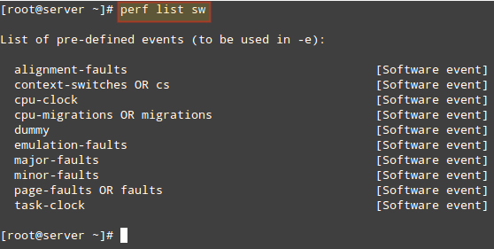
List Software Pre-defined Events in Linux Perf stat
perf stat runs a command and collects Linux performance statistics during the execution of such command. What happens in our system when we run dd
# perf stat dd if=/dev/zero of=test.iso bs=10M count=1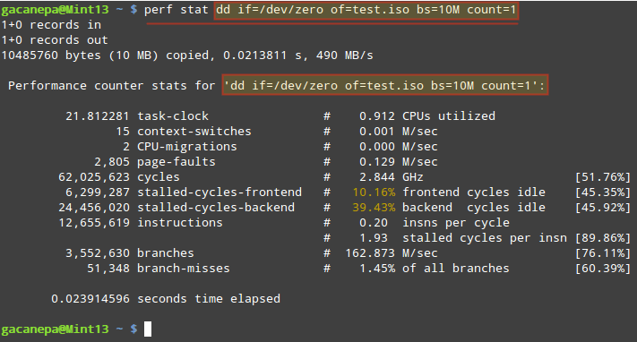
Collects Performance Statistics of Linux Command
The stats shown above indicate, among other things:
- The execution of the dd command took 21.812281 milliseconds of CPU. If we divide this number by the "seconds time elapsed" value below ( 23.914596 milliseconds), it yields 0.912 (CPU utilized).
- While the command was executed, 15 context-switches (also known as process switches) indicate that the CPUs were switched 15 times from one process (or thread) to another.
- CPU migrations is the expected result when in a 2-core CPU the workload is distributed evenly between the number of cores.
During that time ( 21.812281 milliseconds), the total number of CPU cycles that were consumed was 62,025,623 , which divided by 0.021812281 seconds gives 2.843 GHz.- If we divide the number of cycles by the total instructions count we get 4.9 Cycles Per Instruction, which means each instruction took almost 5 CPU cycles to complete (on average). We can blame this (at least in part) on the number of branches and branch-misses (see below), which end up wasting or misusing CPU cycles.
- As the command was executed, a total of 3,552,630 branches were encountered. This is the CPU-level representation of decision points and loops in the code. The more branches, the lower the performance. To compensate for this, all modern CPUs attempt to predict the flow the code will take. 51,348 branch-misses indicate the prediction feature was wrong 1.45% of the time.
The same principle applies to gathering stats (or in other words, profiling) while an application is running. Simply launch the desired application and after a reasonable period of time (which is up to you) close it, and perf will display the stats in the screen. By analyzing those stats you can identify potential problems.
Perf topperf top is similar to top command , in that it displays an almost real-time system profile (also known as live analysis).
With the
-aoption you will display all of the known event types, whereas the-eoption will allow you to choose a specific event category (as returned by perf list ):Will display all cycles event.
perf top -aWill display all cpu-clock related events.
perf top -e cpu-clock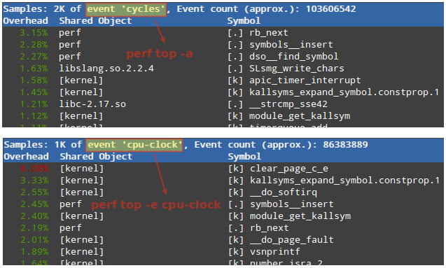
Live Analysis of Linux Performance
The first column in the output above represents the percentage of samples taken since the beginning of the run, grouped by function Symbol and Shared Object. More options are available in man perf-top
Perf recordperf record runs a command and saves the statistical data into a file named perf.data inside the current working directory. It runs similarly to perf stat
Type perf record followed by a command:
# perf record dd if=/dev/null of=test.iso bs=10M count=1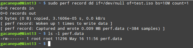
Record Command Statistical Data Perf report
perf report formats the data collected in perf.data above into a performance report:
# sudo perf report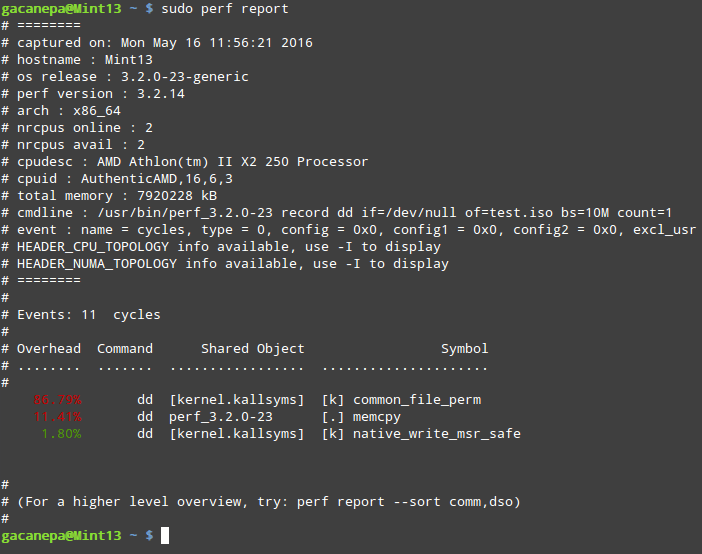
Perf Linux Performance Report
All of the above subcommands have a dedicated man page that can be invoked as:
# man perf-subcommandwhere subcommand is either list , stat top record , or report . These are the most frequently used subcommands; others are listed in the documentation (refer to the Summary section for the link).
SummaryIn this guide we have introduced you to perf , a performance monitoring and analysis tool for Linux. We highly encourage you to become familiar with its documentation which is maintained in https://perf.wiki.kernel.org .
If you find applications that are consuming a high percentage of resources, you may consider modifying the source code, or use other alternatives.
If you have questions about this article or suggestions to improve, we are all ears. Feel free to reach us using the comment form below.
Oct 17, 2017 | linux.die.net
Name
perf-stat - Run a command and gather performance counter statistics
Synopsisperf stat [-e <EVENT> | --event=EVENT] [-a] <command> perf stat [-e <EVENT> | --event=EVENT] [-a] - <command> [<options>]DescriptionThis command runs a command and gathers performance counter statistics from it.
Options<command>...
Examples
- Any command you can specify in a shell.
- -e, --event=
- Select the PMU event. Selection can be a symbolic event name (use perf list to list all events) or a raw PMU event (eventsel+umask) in the form of rNNN where NNN is a hexadecimal event descriptor.
- -i, --no-inherit
- child tasks do not inherit counters
- -p, --pid=<pid>
- stat events on existing process id (comma separated list)
- -t, --tid=<tid>
- stat events on existing thread id (comma separated list)
- -a, --all-cpus
- system-wide collection from all CPUs
- -c, --scale
- scale/normalize counter values
- -r, --repeat=<n>
- repeat command and print average + stddev (max: 100)
- -B, --big-num
- print large numbers with thousands' separators according to locale
- -C, --cpu=
- Count only on the list of CPUs provided. Multiple CPUs can be provided as a comma-separated list with no space: 0,1. Ranges of CPUs are specified with -: 0-2. In per-thread mode, this option is ignored. The -a option is still necessary to activate system-wide monitoring. Default is to count on all CPUs.
- -A, --no-aggr
- Do not aggregate counts across all monitored CPUs in system-wide mode (-a). This option is only valid in system-wide mode.
- -n, --null
- null run - don't start any counters
- -v, --verbose
- be more verbose (show counter open errors, etc)
- -x SEP, --field-separator SEP
- print counts using a CSV-style output to make it easy to import directly into spreadsheets. Columns are separated by the string specified in SEP.
- -G name, --cgroup name
- monitor only in the container (cgroup) called "name". This option is available only in per-cpu mode. The cgroup filesystem must be mounted. All threads belonging to container "name" are monitored when they run on the monitored CPUs. Multiple cgroups can be provided. Each cgroup is applied to the corresponding event, i.e., first cgroup to first event, second cgroup to second event and so on. It is possible to provide an empty cgroup (monitor all the time) using, e.g., -G foo,,bar. Cgroups must have corresponding events, i.e., they always refer to events defined earlier on the command line.
- -o file, --output file
- Print the output into the designated file.
- --append
- Append to the output file designated with the -o option. Ignored if -o is not specified.
- --log-fd
- Log output to fd, instead of stderr. Complementary to --output, and mutually exclusive with it. --append may be used here. Examples: 3>results perf stat --log-fd 3 - $cmd 3>>results perf stat --log-fd 3 --append - $cmd
$ perf stat - make -j
See Also Referenced By perf (1), perf-record (1), perf-report (1) perf-record(1) - Linux man page Name
8117.370256 task clock ticks # 11.281 CPU utilization factor 678 context switches # 0.000 M/sec 133 CPU migrations # 0.000 M/sec 235724 pagefaults # 0.029 M/sec 24821162526 CPU cycles # 3057.784 M/sec 18687303457 instructions # 2302.138 M/sec 172158895 cache references # 21.209 M/sec 27075259 cache misses # 3.335 M/secperf-record - Run a command and record its profile into perf.data
Synopsisperf record [-e <EVENT> | --event=EVENT] [-l] [-a] <command> perf record [-e <EVENT> | --event=EVENT] [-l] [-a] - <command> [<options>]DescriptionThis command runs a command and gathers a performance counter profile from it, into perf.data - without displaying anything.
This file can then be inspected later on, using perf report .
Options<command>...
See Also Referenced By perf (1), perf-annotate (1), perf-archive (1), perf-buildid-cache (1), perf-buildid-list (1), perf-diff (1), perf-evlist (1), perf-inject (1), perf-kmem (1), perf-kvm (1), perf-probe (1), perf-sched (1), perf-script (1), perf-timechart (1)
- Any command you can specify in a shell.
- -e, --event=
- Select the PMU event. Selection can be a symbolic event name (use perf list to list all events) or a raw PMU event (eventsel+umask) in the form of rNNN where NNN is a hexadecimal event descriptor.
- --filter=<filter>
- Event filter.
- -a, --all-cpus
- System-wide collection from all CPUs.
- -l
- Scale counter values.
- -p, --pid=
- Record events on existing process ID (comma separated list).
- -t, --tid=
- Record events on existing thread ID (comma separated list).
- -u, --uid=
- Record events in threads owned by uid. Name or number.
- -r, --realtime=
- Collect data with this RT SCHED_FIFO priority.
- -D, --no-delay
- Collect data without buffering.
- -A, --append
- Append to the output file to do incremental profiling.
- -f, --force
- Overwrite existing data file. (deprecated)
- -c, --count=
- Event period to sample.
- -o, --output=
- Output file name.
- -i, --no-inherit
- Child tasks do not inherit counters.
- -F, --freq=
- Profile at this frequency.
- -m, --mmap-pages=
- Number of mmap data pages. Must be a power of two.
- -g, --call-graph
- Do call-graph (stack chain/backtrace) recording.
- -q, --quiet
- Don't print any message, useful for scripting.
- -v, --verbose
- Be more verbose (show counter open errors, etc).
- -s, --stat
- Per thread counts.
- -d, --data
- Sample addresses.
- -T, --timestamp
- Sample timestamps. Use it with perf report -D to see the timestamps, for instance.
- -n, --no-samples
- Don't sample.
- -R, --raw-samples
- Collect raw sample records from all opened counters (default for tracepoint counters).
- -C, --cpu
- Collect samples only on the list of CPUs provided. Multiple CPUs can be provided as a comma-separated list with no space: 0,1. Ranges of CPUs are specified with -: 0-2. In per-thread mode with inheritance mode on (default), samples are captured only when the thread executes on the designated CPUs. Default is to monitor all CPUs.
- -N, --no-buildid-cache
- Do not update the builid cache. This saves some overhead in situations where the information in the perf.data file (which includes buildids) is sufficient.
- -G name,..., --cgroup name,...
- monitor only in the container (cgroup) called "name". This option is available only in per-cpu mode. The cgroup filesystem must be mounted. All threads belonging to container "name" are monitored when they run on the monitored CPUs. Multiple cgroups can be provided. Each cgroup is applied to the corresponding event, i.e., first cgroup to first event, second cgroup to second event and so on. It is possible to provide an empty cgroup (monitor all the time) using, e.g., -G foo,,bar. Cgroups must have corresponding events, i.e., they always refer to events defined earlier on the command line.
- -b, --branch-any
- Enable taken branch stack sampling. Any type of taken branch may be sampled. This is a shortcut for --branch-filter any. See --branch-filter for more infos.
- -j, --branch-filter
- Enable taken branch stack sampling. Each sample captures a series of consecutive taken branches. The number of branches captured with each sample depends on the underlying hardware, the type of branches of interest, and the executed code. It is possible to select the types of branches captured by enabling filters. The following filters are defined:
- Б─╒ any: any type of branches
- Б─╒ any_call: any function call or system call
- Б─╒ any_ret: any function return or system call return
- Б─╒ ind_call: any indirect branch
- Б─╒ u: only when the branch target is at the user level
- Б─╒ k: only when the branch target is in the kernel
- Б─╒ hv: only when the target is at the hypervisor level
- The option requires at least one branch type among any, any_call, any_ret, ind_call. The privilege levels may be ommitted, in which case, the privilege levels of the associated event are applied to the branch filter. Both kernel (k) and hypervisor (hv) privilege levels are subject to permissions. When sampling on multiple events, branch stack sampling is enabled for all the sampling events. The sampled branch type is the same for all events. The various filters must be specified as a comma separated list: --branch-filter any_ret,u,k Note that this feature may not be available on all processors.
Oct 15, 2017 | sourceforge.net
- Vladimir Rybkin committed [r18078]
added test dependence on another test in embedding
- 2 days ago
Vladimir Rybkin committed [r18077]
changed the test reference
- 2 days ago
Vladimir Rybkin committed [r18076]
changed the test failing with farming
- 11 days ago
Vladimir Rybkin committed [r18075]
fixed constant potential and added a test
- 11 days ago
Juerg Hutter committed [r18074]
Eva Perlt (Bonn): new B97 paramtrization + short range D3 correction
- 11 days ago
Andreas Gloess committed [r18073]
VDW-corr: Adjust tolerance.
- 12 days ago
Vladimir Rybkin committed [r18072]
enable restart with embedding
- 13 days ago
Juerg Hutter committed [r18071]
Bug fix: Grimme D3 C9 term: use original parameter
- 14 days ago
Nico Holmberg committed [r18070]
CDFT: Tidy input descriptions
Oct 14, 2017 | www.collabora.com
Posted on 21/03/2017 by Gabriel Krisman Bertazi
Dynamic profilers are tools to collect data statistics about applications while they are running, with minimal intrusion on the application being observed.
The kind of data that can be collected by profilers varies deeply, depending on the requirements of the user. For instance, one may be interested in the amount of memory used by a specific application, or maybe the number of cycles the program executed, or even how long the CPU was stuck waiting for data to be fetched from the disks. All this information is valuable when tracking performance issues, allowing the programmer to identify bottlenecks in the code, or even to learn how to tune an application to a specific environment or workload.
In fact, maximizing performance or even understanding what is slowing down your application is a real challenge on modern computer systems. A modern CPU carries so many hardware techniques to optimize performance for the most common usage case, that if an application doesn't intentionally exploit them, or worse, if it accidentally lies in the special uncommon case, it may end up experiencing terrible results without doing anything apparently wrong.
Let's take a quite non-obvious way of how things can go wrong, as an example.
Forcing branch mispredictionsBased on the example from here .
The code below is a good example of how non-obvious performance assessment can be. In this function, the first for loop initializes a vector of size n with random values ranging from 0 to N. We can assume the values are well distributed enough for the vector elements to be completely unsorted.
The second part of the code has a for loop nested inside another one. The outer loop, going from 0 to K, is actually a measurement trick. By executing the inner loop many times, it stresses out the performance issues in that part of the code. In this case, it helps to reduce any external factor that may affect our measurement.
The inner loop is where things get interesting. This loop crawls over the vector and decides whether the value should be accumulated in another variable, depending on whether the element is higher than N/2 or not. This is done using an if clause, which gets compiled into a conditional branch instruction, which modifies the execution flow depending on the calculated value of the condition, in this case, if vec[i] >= N/2, it will enter the if leg, otherwise it will skip it entirely.
long rand_partsum(int n)
{
  int i,k;
  long sum = 0;
  int *vec = malloc(n * sizeof(int));

  for (i = 0; i < n; i++)
    vec[i] = rand()%n;

  for (k = 0; k < 1000000; k++)
    for (i = 0; i < n; i++)
      if (vec[i] > n/2)
        sum += vec[i];

  return sum;
}
When executing the code above on an Intel Core i7-5500U, with a vector size of 5000 elements (N=5000), it takes an average of 29.97 seconds. Can we do any better?One may notice that this vector is unsorted, since each element comes from a call to rand(). What if we sorted the vector before executing the second for loop? For the sake of the example, let's say we add a call to the glibc implementation of QuickSort right after the initialization loop.
A naive guess would suggest that the algorithm got worse, because we just added a new sorting step, thus raising the complexity of the entire code. One should assume this would result on a higher execution time.
But, in fact, when executing the sorted version in the same machine, the average execution time drops to 13.20 seconds, which is a reduction of 56% in execution time. Why does adding a new step actually reduces the execution time? The fact is that pre-sorting the vector in this case, allows the cpu to do a much better job at internally optimizing the code during execution. In this case, the issue observed was a high number of branch mispredictions, which were triggered by the conditional branch that implements the if clause.
Modern CPUs have quite deep pipelines, meaning that the instruction being fetched on any given cycle is always a few instructions down the road than the instruction actually executed on that cycle. When there is a conditional branch along the way, there are two possible paths that can be followed, and the prefetch unit has no idea which one it should choose, until all the actual condition for that instruction is calculated.
The obvious choice for the Prefetch unit on such cases is to stall and wait until the execution unit decides the correct path to follow, but stalling the pipeline like this is very costly. Instead, a speculative approach can be taken by a unit called Branch Predictor, which tries to guess which path should be taken. After the condition is calculated, the CPU verifies the guessed path: if it got the prediction right, in other words, if a branch prediction hit occurs, the execution just continues without much performance impact, but if it got it wrong, the processor needs to flush the entire pipeline, go back, and restart executing the correct path. The later is called a branch prediction miss, and is also a costly operation.
In systems with a branch predictor, like any modern CPU, the predictor is usually based on the history of the particular branches. If a conditional branch usually goes a specific way, the next time it appears, the predictor will assume it will take the same route.
Back to our example code, that if condition inside the for loop does not have any specific pattern. Since the vector elements are completely random, sometimes it will enter the if leg, sometimes it will skip it entirely. That is a very hard situation for the branch predictor, who keeps guessing wrong and triggering flushes in the pipeline, which keeps delaying the application.
In the sorted version, instead, it is very easy to guess whether it should enter the if leg or not. For the first part of the vector, where the elements are mostly < N/2, the if leg will always be skipped, while for the second part, it will always enter the if leg. The branch predictor is capable of learning this pattern after a few iterations, and is able to do much better guesses about the flow, reducing the number of branch misses, thus increasing the overall performance.
Well, pointing specific issues like this is usually hard, even for a simple code like the example above. How could we be sure that the the program is hitting enough branch mispredictions to affect performance? In fact, there are always many things that could be the cause of slowness, even for a slightly more complex program.
Perf_events is an interface in the Linux kernel and a userspace tool to sample hardware and software performance counters. It allows, among many other things, to query the CPU register for the statistics of the branch predictor, i.e. the number of prediction hits and misses of a given application.
The userspace tool, known as the perf command, is available in the usual channels of common distros. In Debian, for instance, you can install it with:
We'll dig deeper into the perf tool later on another post, but for now, let's use the, perf record and perf annotate commands, which allow tracing the program and annotating the source code with the time spent on each instruction, and the perf stat command, which allows to run a program and display statistics about it:
At first, we can instruct perf to instrument the program and trace its execution:
The perf record will execute the program passed as parameter and collect performance information into a new perf.data file. This file can then be passed to other perf commands. In this case, we pass it to the perf annotate command, which crawls over each address in the program and prints the number of samples that was collected while the program was executing each instruction. Instructions with a higher number of samples indicates that the program spent more time in that region, indicating that it is hot code, and a good part of the program to try to optimize. Notice that, for modern processors, the exact position is an estimation, so this information must be used with care. As a rule of thumb, one should be looking for hot regions, instead of single hot instructions.Below is the output of perf annotate, when analyzing the function above. The output is truncated to display only the interesting parts.
[krisman@dilma bm]$ perf annotate

        :
        :      int rand_partsum()
        :      {
   0.00 :        74e:   push   %rbp
   0.00 :        74f:   mov    %rsp,%rbp
   0.00 :        752:   push   %rbx
   0.00 :        753:   sub    $0x38,%rsp
   0.00 :        757:   mov    %rsp,%rax
   0.00 :        75a:   mov    %rax,%rbx

   [...]

   0.00 :        7ce:   mov    $0x0,%edi
   0.00 :        7d3:   callq  5d0 <time@plt>
   0.00 :        7d8:   mov    %eax,%edi
   0.00 :        7da:   callq  5c0 <srand@plt>
        :              for (i = 0; i < n; i++)
   0.00 :        7df:   movl   $0x0,-0x14(%rbp)
   0.00 :        7e6:   jmp    804 <main+0xb6>
        :                      vec[i] = rand()%n;
   0.00 :        7e8:   callq  5e0 <rand@plt>
   0.00 :        7ed:   cltd
   0.00 :        7ee:   idivl  -0x24(%rbp)
   0.00 :        7f1:   mov    %edx,%ecx
   0.00 :        7f3:   mov    -0x38(%rbp),%rax
   0.00 :        7f7:   mov    -0x14(%rbp),%edx
   0.00 :        7fa:   movslq %edx,%rdx
   0.00 :        7fd:   mov    %ecx,(%rax,%rdx,4)
        :              for (i = 0; i < n; i++)
   0.00 :        800:   addl   $0x1,-0x14(%rbp)
   0.00 :        804:   mov    -0x14(%rbp),%eax
   0.00 :        807:   cmp    -0x24(%rbp),%eax
   0.00 :        80a:   jl     7e8 <main+0x9a>

   [...]

         :              for (k = 0; k < 1000000; k++)
    0.00 :        80c:   movl   $0x0,-0x18(%rbp)
    0.00 :        813:   jmp    85e <main+0x110>
         :                      for (i = 0; i < n; i++)
    0.01 :        815:   movl   $0x0,-0x14(%rbp)
    0.00 :        81c:   jmp    852 <main+0x104>
         :                              if (vec[i] > n/2)
    0.20 :        81e:   mov    -0x38(%rbp),%rax
    6.47 :        822:   mov    -0x14(%rbp),%edx
    1.94 :        825:   movslq %edx,%rdx
   26.86 :        828:   mov    (%rax,%rdx,4),%edx
    0.08 :        82b:   mov    -0x24(%rbp),%eax
    1.46 :        82e:   mov    %eax,%ecx
    0.62 :        830:   shr    $0x1f,%ecx
    3.82 :        833:   add    %ecx,%eax
    0.06 :        835:   sar    %eax
    0.70 :        837:   cmp    %eax,%edx
    0.42 :        839:   jle    84e <main+0x100>
         :                                      sum += vec[i];
    9.15 :        83b:   mov    -0x38(%rbp),%rax
    5.91 :        83f:   mov    -0x14(%rbp),%edx
    0.26 :        842:   movslq %edx,%rdx
    5.87 :        845:   mov    (%rax,%rdx,4),%eax
    2.09 :        848:   cltq
    9.31 :        84a:   add    %rax,-0x20(%rbp)
         :                      for (i = 0; i < n; i++)
   16.66 :        84e:   addl   $0x1,-0x14(%rbp)
    6.46 :        852:   mov    -0x14(%rbp),%eax
    0.00 :        855:   cmp    -0x24(%rbp),%eax
    1.63 :        858:   jl     81e <main+0xd0>
         :              for (k = 0; k < 1000000; k++)

   [...]
The first thing to notice is that the perf command tries to interleave C code with the Assembly code. This feature requires compiling the test program with -g3 to include debug information.
The number before the ':' is the percentage of samples collected while the program was executing each instruction. Once again, this is not an exact information, so you should be looking for hot regions, and not specific instructions.
The first and second hunk are the function prologue, which was executed only once, and the vector initialization. According to the profiling data, there is little point in attempting to optimize them, because the execution practically didn't spend any time on it. The third hunk is the second loop, where it spent almost all the execution time. Since that loop is where most of our samples where collected, we can assume that it is a hot region, which we can try to optimize. Also, notice that most of the samples were collected around that if leg. This is another indication that we should look into that specific code.
To find out what might be causing the slowness, we can use the perf stat command, which prints a bunch of performance counters information for the entire program. Let's take a look at its output.
[krisman@dilma bm]$ perf stat ./branch-miss.unsorted

 Performance counter stats for './branch-miss.unsorted:

    29876.773720  task-clock (msec) #    1.000 CPUs utilized
              25  context-switches  #    0.001 K/sec
               0  cpu-migrations    #    0.000 K/sec
              49  page-faults       #    0.002 K/sec
  86,685,961,134  cycles            #    2.901 GHz
  90,235,794,558  instructions      #    1.04  insn per cycle
  10,007,460,614  branches          #  334.958 M/sec
   1,605,231,778  branch-misses     #   16.04% of all branches

   29.878469405 seconds time elapsed
Perf stat will dynamically profile the program passed in the command line and report back a number of statistics about the entire execution. In this case, let's look at the 3 last lines in the output. The first one gives the rate of instructions executed per CPU cycle; the second line, the total number of branches executed; and the third, the percentage of those branches that resulted in a branch miss and pipeline flush.Perf is even nice enough to put important or unexpected results in red. In this case, the last line, Branch-Misses, was unexpectedly high, thus it was displayed in red in this test.
And now, let's profile the pre-sorted version. Look at the number of branch misses:
[krisman@dilma bm]$ perf stat ./branch-miss.sorted

 Performance counter stats for './branch-miss.sorted:

    14003.066457  task-clock (msec) #    0.999 CPUs utilized
             175  context-switches  #    0.012 K/sec
               4  cpu-migrations    #    0.000 K/sec
              56  page-faults       #    0.004 K/sec
  40,178,067,584  cycles            #    2.869 GHz
  89,689,982,680  instructions      #    2.23  insn per cycle
  10,006,420,927  branches          #  714.588 M/sec
       2,275,488  branch-misses     #    0.02% of all branches

  14.020689833 seconds time elapsed
It went down from over 16% to just 0.02% of the total branches! This is very impressive and is likely to explain the reduction in execution time. Another interesting value is the number of instructions per cycle, which more than doubled. This happens because, once we reduced the number of stalls, we make better use of the pipeline, obtaining a better instruction throughput. Wrapping upAs demonstrated by the example above, figuring out the root cause of a program slowness is not always easy. In fact, it gets more complicated every time a new processor comes out with a bunch of shiny new optimizations.
Despite being a short example code, the branch misprediction case is still quite non-trivial for anyone not familiar with how the branch prediction mechanism works. In fact, if we just look at the algorithm, we could have concluded that adding a sort algorithm would just add more overhead to the algorithm. Thus, this example gives us a high-level view of how helpful profiling tools really are. By using just one of the several features provided by the perf tool, we were able to draw major conclusions about the program being examined.
Comments (10)Performance analysis in Linux (continued)
Alan:
sum += n[i];
Apr 03, 2017 at 11:46 AM
should be
sum += vec[i];
![]()
Krisman:
Thanks Alan. That's correct, I've fixed it now.
Apr 03, 2017 at 01:47 PM![]()
Arvin :
Thank you for the excellent write-up, Krisman. For those following along, I was able to grab perf for my current kernel on Ubuntu with the following command: sudo apt install linux-tools-`uname -r`
Apr 03, 2017 at 06:08 PMI was amazed at how well the -O3 compiler option was over -O2 and below with the unsorted code (-O2, -O1, and without were pretty much the same interestingly enough).
Is this essentially doing under-the-hood what the sorted code is doing? Or is the compiler using other tricks to drastically improve performance here? Thanks again!
![]()
krisman:
The compiler is likely not sorting the vector, because it can't be sure such transformation would be correct or even helpful. But, which optimization it actually applies when increasing the optimization level depends on the compiler you have and which exact version you used. It may try, for instance, unrolling the loop
Apr 03, 2017 at 08:03 PM
to use more prediction slots, though I don't think it would make a difference here.A higher optimization level could also eliminate that outer loop, should it conclude it is useless for calculating the overall sum. To find out what happened in your
case, you might wish to dump the binary with a tool like objdump and checkout the generated assembly for clues.gcc -O3 main.c -o branch-miss
objdump -D branch-miss | lessIn my system, when compiling with -O3, gcc was able to optimize that inner loop with vector instructions, which eliminated most of the branch misses.
In the second perf stat you shared, you can see that the result was similar, it drastically reduced the number of branch misses, resulting in an increase of the instructions per cycle rate.
Arvin:
Interesting, thanks! I'll keep playing with it. I was also curious how clang compared. Same number of branch misses, but many more instructions! Notable increase in execution time.
Apr 03, 2017 at 10:17 PMAll in all, this was fun and I learned something new today :)
Anon:
The optimisation change that flattens the results is explained in the most popular stack overflow answer ever: http://stackoverflow.com/a/11227902
Apr 06, 2017 at 07:50 AMThomas:
Nice post, thanks for sharing.
Apr 03, 2017 at 06:39 PM
The return type of rand_partsum() should be long though to match the variable sum.
krisman:
Thanks! fixed that as well.
Apr 03, 2017 at 08:05 PM![]()
Solerman Kaplon:
how does the perf annotate looks like in the sort version? I'm curious how the cpu would understand that the data is sorted, never heard of such a thing
Apr 03, 2017 at 08:56 PM
![]()
krisman:
Hi Solerman,
Apr 04, 2017 at 01:42 AMIt's not that the CPU understands the data is sorted, it doesn't. Instead, we use the knowledge acquired with perf to assemble the data in a specific way to explore the characteristics of the processor.
In this case, we prepared the data in a way that made the conditional branch taken by the 'if' clause predictable for a history-based branch predictor, like the ones in modern cpus. By sorting the data, we ensure the first part of the array will always skip the 'if' leg, while the second part will always enter the 'if' leg. There might still be branch misses, when entering the vector and when switching from the first part of the vector to the second, for instance. But those branch misses are
negligible since, by puting some order in the data, we ensured the vast majority of iterations won't trigger mispredictions.The expectation for the perf annotation of the optimized version would be a more even distribution of samples along the program code. If we only have this function alone in our program, it's likely that most samples will still be in the nested loops since that is, by far, the hottest path in our simple program. But
even then, the optimized version may still have a slightly better distribution of samples, since we don't waste too much time stalled on that conditional branch. In the article example, perf annotate allowed us to isolate the region that made the most sense trying to optimize, which are always the parts where the execution
spends most time.06/10/2017
In this post, I will show one more example of how easy it is to disrupt performance of a modern CPU, and also run a quick discussion on
XDC 2017 - Links to recorded presentations (videos)23/09/2017
Many thanks to Google for recording all the XDC2017 talks. To make them easier to watch, here are direct links to each talk recorded at
DebConf 17: Flatpak and Debian17/08/2017
Last week, I attended DebConf 17 in Montréal, returning to DebConf for the first time in 10 years (last time was DebConf 7 in Edinburgh).
Android: NXP i.MX6 on Etnaviv Update24/07/2017
More progress is being made in the area of i.MX6, etnaviv and Android. Since the last post a lot work has gone into upstreaming and stabilizing
vkmark: more than a Vulkan benchmark18/07/2017
Ever since Vulkan was announced a few years ago, the idea of creating a Vulkan benchmarking tool in the spirit of glmark2 had been floating
Quick hack: Performance debugging Linux graphics on Mesa29/06/2017
Debugging graphics performance in a simple and high-level manner is possible for all Gallium based Mesa drivers using GALLIUM_HUD, a feature About Collabora
Whether writing a line of code or shaping a longer-term strategic software development plan, we'll help you navigate the ever-evolving world of Open Source.
Jul 28, 2017 | hpc.nrel.gov
- Contents
Instructions and policies for installing and maintaining environment modules on Peregrine.
Toolchains:Libraries and applications are built around the concept of 'toolchains'; at present a toolchain is defined as a specific version of a compiler and MPI library or lack thereof. Applications are typically built with only a single toolchain, whereas libraries are built with and installed for potentially multiple toolchains as necessary to accommodate ABI differences produced by different toolchains. Workflows are primarily composed of the execution of a sequence of applications which may use different tools and might be orchestrated by an application or other tool. The toolchains presently supported are:
- impi-intel
- openmpi-gcc
- comp-intel (no MPI)
- gcc (no MPI)
Loading one of the above MPI-compiler modules will also automatically load the associated compiler module (currently gcc 4.8.2 and comp-intel/13.1.3 are the recommended compilers). Certain applications may of course require alternative toolchains. If demand for additional options becomes significant, requests for additional toolchain support will be considered on a case-by-case basis.
Building Module Files Here are the steps for building an associated environment module for the installed mysoft software. First, create the appropriate module location% mkdir -p /nopt/nrel/apps/modules/candidate/modulefiles/mysoft # Use a directory and not a file. % touch /nopt/nrel/apps/modules/candidate/modulefiles/mysoft/1.3 # Place environment module tcl code here. % touch .version # If required, indicate default module in this file.Next, edit the module file itself ("1.3" in the example). The current version of the HPC Standard Module Template is:#%Module -*- tcl -*- # Specify conflicts # conflict 'appname' # Prerequsite modules # prereq 'appname/version....' #################### Set top-level variables ######################### # 'Real' name of package, appears in help,display message set PKG_NAME pkg_name # Version number (eg v major.minor.patch) set PKG_VERSION pkg_version # Name string from which enviro/path variable names are constructed # Will be similar to, be not necessarily the same as, PKG_NAME # eg PKG_NAME-->VisIt PKG_PREFIX-->VISIT set PKG_PREFIX pkg_prefix # Path to the top-level package install location. # Other enviro/path variable values constructed from this set PKG_ROOT pkg_root # Library name from which to construct link line # eg PKG_LIBNAME=fftw ---> -L/usr/lib -lfftw set PKG_LIBNAME pkg_libname ###################################################################### proc ModulesHelp { } { global PKG_VERSION global PKG_ROOT global PKG_NAME puts stdout "Build: $PKG_NAME-$PKG_VERSION" puts stdout "URL: http://www.___________" puts stdout "Description: ______________________" puts stdout "For assistance contact [email protected]" } module-whatis "$PKG_NAME: One-line basic description" # # Standard install locations # prepend-path PATH $PKG_ROOT/bin prepend-path MANPATH $PKG_ROOT/share/man prepend-path INFOPATH $PKG_ROOT/share/info prepend-path LD_LIBRARY_PATH $PKG_ROOT/lib prepend-path LD_RUN_PATH $PKG_ROOT/lib # # Set environment variables for configure/build # ##################### Top level variables ########################## setenv ${PKG_PREFIX} "$PKG_ROOT" setenv ${PKG_PREFIX}_ROOT "$PKG_ROOT" setenv ${PKG_PREFIX}_DIR "$PKG_ROOT" #################################################################### ################ Template include directories ###################### # Only path names setenv ${PKG_PREFIX}_INCLUDE "$PKG_ROOT/include" setenv ${PKG_PREFIX}_INCLUDE_DIR "$PKG_ROOT/include" # 'Directives' setenv ${PKG_PREFIX}_INC "-I $PKG_ROOT/include" #################################################################### ################## Template library directories #################### # Only path names setenv ${PKG_PREFIX}_LIB "$PKG_ROOT/lib" setenv ${PKG_PREFIX}_LIBDIR "$PKG_ROOT/lib" setenv ${PKG_PREFIX}_LIBRARY_DIR "$PKG_ROOT/lib" # 'Directives' setenv ${PKG_PREFIX}_LD "-L$PKG_ROOT/lib" setenv ${PKG_PREFIX}_LIBS "-L$PKG_ROOT/lib -l$PKG_LIBNAME" ####################################################################
- The tags 'pkg_name', 'pkg_version', 'pkg_prefix', 'pkg_root' and 'pkg_libname' should be replaced by the appropriate names for the library or application.
- Specify any module prerequisites and/or conflicts.
- Provide content for the URL and Description in the 'ModulesHelp' procedure
- Give a one-line description for the 'module whatis' line. This should reflect pkg_name, pkg_version, and the toolchain used to build.
- If needed, augment or edit the pre-defined environment settings (Note: the default procedure is to use ' prepend-path to permit bottom-up construction of an environment stack ).
- The ${PKG_PREFIX}_LIBS variable could require manual changes by developers due to non-standard and/or multiple library names.
The current module file template is maintained in a version control repo at [email protected]:hpc/hpc-devel.git. The template file is located in hpc-devel/modules/modTemplate . To see the current file
git clone [email protected]:hpc/hpc-devel.git
cd ./hpc-devel/modules/
cat modTemplate
Next specify a default version of the module package. Here is an example of an an associated .version file for a set of module files
% cat /nopt/nrel/apps/modules/candidate/modulefiles/mysoft/.version
#%Module########################################
# vim: syntax=tcl

set ModulesVersion "1.3"
The .version file is only useful if there are multiple versions of the software installed. Put notes in the modulefile as necessary in stderr of the modulefile for the user to use the software correctly and for additional pointers.
NOTE : For modules with more than one level of sub-directory, although the default module as specified above is displayed correctly by the modules system, it is not loaded correctly!if more than one version exists, the most recent one will be loaded by default. In other words, the above will work fine for dakota/5.3.1 if 5.3.1 is a file alongside the file dakota/5.4 , but not for dakota/5.3.1/openmpi-gcc when a dakota/5.4 directory is present. In this case, to force the correct default module to be loaded, a dummy symlink needs to be added in dakota/ that points to the module specified in .version
Example
% cat /nopt/nrel/apps/modules/default/modulefiles/dakota/.version
#%Module########################################
# vim: syntax=tcl

set ModulesVersion "5.3.1/openmpi-gcc"

% module avail dakota
------------------------------------------------------------------ /nopt/nrel/apps/modules/default/modulefiles -------------------------------------------------------------------
dakota/5.3.1/impi-intel           dakota/5.3.1/openmpi-epel         dakota/5.3.1/openmpi-gcc(default) dakota/5.4/openmpi-gcc            dakota/default

% ls -l /nopt/nrel/apps/modules/default/modulefiles/dakota
total 8
drwxrwsr-x 2 ssides   n-apps 8192 Sep 22 13:56 5.3.1
drwxrwsr-x 2 hsorense n-apps   96 Jun 19 10:17 5.4
lrwxrwxrwx 1 cchang   n-apps   17 Sep 22 13:56 default -> 5.3.1/openmpi-gcc
Naming ModulesSoftware which is made accessible via the modules system generally falls into one of three categories.
- Applications: these may be intended to carry out scientific calculations, or tasks like performance profiling of codes.
- Libraries: collections of header files and object code intended to be incorporated into an application at build time, and/or accessed via dynamic loading at runtime. The principal exceptions are technical communication libraries such as MPI, which are categorized as toolchain components below.
- Toolchains: compilers (e.g., Intel, GCC, PGI) and MPI libraries (OpenMPI, IntelMPI, mvapich2).
Often a package will contain both executable files and libraries. Whether it is classified as an Application or a Library depends on its primary mode of utilization. For example, although the HDF5 package contains a variety of tools for querying HDF5-format files, its primary usage is as a library which applications can use to create or access HDF5-format files. Each package can also be distinguished as a vendor- or developer-supplied binary, or a collection of source code and build components ( e.g. , Makefile(s)).
For pre-built applications or libraries, or for applications built from source code, the basic form of the module name should be
{package_name}/{version}. For libraries built from source, or any package containing components which can be linked against in normal usage, the name should be
{package_name}/{version}/{toolchain}The difference arises from two considerations. For supplied binaries, the assumed vendor or developer expectation is that a package will run either on a specified Linux distribution (and may have specific requirements satisfied by the distribution), or across varied distributions (and has fairly generic requirements satisfied by most or all distributions). Thus, the toolchain for supplied binaries is implicitly supplied by the operating system. For source code applications, the user should not be directly burdened with the underlying toolchain requirement; where this is relevant ( i.e. , satisfying dependencies), the associated information should be available in module help output, as well as through dependency statements in the module itself.
Definitions:
{package_name} : This should be chosen such that the associated Application, Library, or Toolchain component is intuitively obvious, while concomitantly distinguishing its target from other Applications, Libraries, or Toolchain components likely to be made available on the system through the modules. So, "gaussian" is a sensible package_name , whereas "gsn" would be too generic and of unclear intent. Within these guidelines, though, there is some discretion left to the module namer.
{version} : The base version generally reflects the state of development of the underlying package, and is supplied by the developers or vendor. However, a great deal of flexibility is permitted here with respect to build options outside of the recognized {toolchain} terms. So, a Scalapack-enabled package version might be distinguished from a LAPACK-linked one by appending "-sc" to the base version, provided this is explained in the "module help" or "module show" information. {version} provides the most flexibility to the module namer.
{toolchain} : This is solely intended to track the compiler and MPI library used to build a source package. It is not intended to track the versions of these toolchain components, nor to track the use of associated toolkits ( e.g. , Cilk Plus) or libraries ( e.g. , MKL, Scalapack). As such, this term takes the form {MPI}-{compiler} , where {MPI} is one of
- openmpi
- impi (Intel MPI)
and {compiler} is one of
Module Directory Organization For general support, modulefiles can be installed in three top locations:
- gcc
- intel
- epel (which implies the gcc supplied with the OS, possibly at a newer version number than that in the base OS exposed in the filesystem without the EPEL module).
- /nopt/Modules/3.2.10/modulefiles (Modules supplied by HP, not supported by the HPC Modeling & Simulation group)
- /nopt/nrel/apps/modules (majority of modules, most common location)
- /nopt/nrel/ecom/modules (specialized modules for certain groups/applications)
In addition, more specific requests can be satisfied in two other ways:
For the '/nopt/nrel/apps' modules location (where most general installations should be made), the following sub-directories have been created:
- /projects/X/modules (Modules useful to a single project with allocated resource)
- /home/$USER/modules (Modules useful to a single user)
to manage how modules are developed, tested and provided for production level use. An example directory hierarchy for the module files is as follows:
- /nopt/nrel/apps/modules/candidate/modulefiles
- /nopt/nrel/apps/modules/default/modulefiles
- /nopt/nrel/apps/modules/deprecated/modulefiles
- /nopt/nrel/apps/modules/hpc/modulefiles
[wjones@login2 nrel]$ tree -a apps/modules/default/modulefiles/hdf5-parallel/
apps/modules/default/modulefiles/hdf5-parallel/
├── .1.6.4
│   ├── impi-intel
│   ├── openmpi-gcc
│   └── .version
├── 1.8.11
│   ├── impi-intel
│   └── openmpi-gcc
└── .version

[wjones@login2 nrel]$ tree -a apps/modules/default/modulefiles/hdf5
apps/modules/default/modulefiles/hdf5
├── .1.6.4
│   └── intel
├── 1.8.11
│   ├── gcc
│   └── intel
└── .version

[wjones@login2 nrel]$ module avail hdf5

------------------------------------------------------- /nopt/nrel/apps/modules/default/modulefiles -------------------------------------------------------
hdf5/1.8.11/gcc                          hdf5-parallel/1.8.11/impi-intel(default)
hdf5/1.8.11/intel(default)               hdf5-parallel/1.8.11/openmpi-gcc
Module Migrationlast modified Jul 06, 2015 03:16 PM
- There are three file paths for which this document is intended. Each corresponds to a status of modules within a broader workflow for managing modules. (The other module locations are not directly part of the policy).
- /nopt/nrel/apps/modules/candidate/modulefiles : This is the starting point for new modules. Modules are to be created here for testing and validation prior to production release. Modules here are not necessarily expected to work without issues, and may be modified or deleted without warning.
- /nopt/nrel/apps/modules/default/modulefiles : This is the production location, visible to the general user community by default. Modules here carry the expectation of functioning properly. Movement of modulefiles into and out of this location is managed through a monthly migration process.
- /nopt/nrel/apps/modules/deprecated/modulefiles : This location contains older modules which are intended for eventual archiving. Conflicts with newer software may render these modules non-functional, and so there is not an expectation of maintenance for these. They are retained to permit smooth migration out of the Peregrine software stack ( i.e. , users will still have access to them and may register objections/issues while retaining their productivity).
- "modifications" to modules entail
- Additions to any of the three stages;
- Major changes in functionality for modules in /default or /deprecated;
- Archiving modules from /deprecated; or,
- Making a module "default"
These are the only acceptable atomic operations. Thus, a migration is defined as an addition to one path and a subsequent deletion from its original path.
- Announcements to users may be one of the following six options:
- Addition to /candidate!"New Module";
- Migration from /candidate to /default!"Move to Production";
- Migration from /default to /deprecated!"Deprecate";
- Removing visibility and accessibility from /deprecated!"Archive"; or,
- Major change in functionality in /default or /deprecated!"Modify"
- Make default!"Make default"
Changes outside of these options, e.g. , edits in /candidate, will not be announced as batching these changes would inhibit our ability to respond nimbly to urgent problems.
- A "major change in functionality" is an edit to the module that could severely compromise users' productivity in the absence of adaptation on their part. So, pointing to a different application binary could result in incompatibilities in datasets generated before and after the module change; changing a module name can break workflows over thousands of jobs. On the other hand, editing inline documentation, setting an environment variable that increases performance with no side effects, or changing a dependency maintenance revision (e.g., a secondary module load of a library from v3.2.1 to v3.2.2) is unlikely to create major problems and does not need explicit attention.
- All module modifications are to be documented in the Sharepoint Modules Modifications table prior to making any changes (this table is linked at http://cs.hpc.nrel.gov/modeling/hpc-sharepoint-assets).
- Module modifications are to be batched for execution on monthly calendar boundaries, and (a) announced to [email protected] two weeks prior to execution, and (b) added to http://hpc.nrel.gov/users/announcements as a new page, which will auto-populate the table visible on the front page. Endeavor to make this list final prior to the first announcement.
- Modules may not be added to or deleted from /default without a corresponding deletion/addition from one of the other categories, i.e. , they may only be migrated relative to /default, not created or deleted directly.
- Good faith testing. There is not currently a formally defined testing mechanism for new modules in /candidate. It is thus left to the individual module steward's (most likely the individual who owns the modulefile in the *NIX sense) discretion what is a defensible test regimen. Within the current document's scope, this specifically relates to the module functionality, not the application functionality.
- Library and toolchain dependencies must be checked for prior to removal of modules from .../deprecated. For example, if a user identifies an application dependency on a deprecated library or toolchain, then the application module will point to the specific library or toolchain version!if it were not, then presumably an updated library/toolchain would be breaking the application. Thus, checking for dependencies on deprecated versions can be done via simple grep of all candidate and production modules. (An obvious exception is if the user is handling the dependencies in their own scripts; this case can not be planned around). It is assumed that an identified dependency on a deprecated module would spur rebuilding and testing of the application against newer libraries/toolchain, so that critical dependency on deprecated tools may not often arise in practice.
Jul 28, 2017 | genomics.upenn.edu
Basic module usageTo know what modules are available, you'll need to run the "module avail" command from an interactive session:
[asrini@consign ~]$ bsub -Is bash
Job <9990024> is submitted to default queue <interactive>.
<<Waiting for dispatch ...>>
<<Starting on node063.hpc.local>>

[asrini@node063 ~]$ module avail

------------------------------------------------------------------- /usr/share/Modules/modulefiles -------------------------------------------------------------------
NAMD-2.9-Linux-x86_64-multicore dot                             module-info                     picard-1.96                     rum-2.0.5_05
STAR-2.3.0e                     java-sdk-1.6.0                  modules                         pkg-config-path                 samtools-0.1.19
STAR-hg19                       java-sdk-1.7.0                  mpich2-x86_64                   python-2.7.5                    use.own
STAR-mm9                        ld-library-path                 null                            r-libs-user
bowtie2-2.1.0                   manpath                         openmpi-1.5.4-x86_64            ruby-1.8.7-p374
devtoolset-2                    module-cvs                      perl5lib                        ruby-1.9.3-p448
The module names should be pretty self-explainatory, but some are not. To see information about a module you can issue a module show [module name] :[asrini@node063 ~]$ module show null ------------------------------------------------------------------- /usr/share/Modules/modulefiles/null: module-whatis does absolutely nothing ------------------------------------------------------------------- [asrini@node063 ~]$ module show r-libs-user ------------------------------------------------------------------- /usr/share/Modules/modulefiles/r-libs-user: module-whatis Sets R_LIBS_USER=$HOME/R/library setenv R_LIBS_USER ~/R/library ------------------------------------------------------------------- [asrini@node063 ~]$ module show devtoolset-2 ------------------------------------------------------------------- /usr/share/Modules/modulefiles/devtoolset-2: module-whatis Devtoolset-2 packages include the newer versions of gcc prepend-path PATH /opt/rh/devtoolset-2/root/usr/bin prepend-path MANPATH /opt/rh/devtoolset-2/root/usr/share/man prepend-path INFOPATH /opt/rh/devtoolset-2/root/usr/share/info -------------------------------------------------------------------Example use of modules:
[asrini@node063 ~]$ python -V
Python 2.6.6

[asrini@node063 ~]$ which python
/usr/bin/python

[asrini@node063 ~]$ module load python-2.7.5

[asrini@node063 ~]$ python -V
Python 2.7.5

[asrini@node063 ~]$ which python
/opt/software/python/python-2.7.5/bin/python
After running the above commands, you will be able to use python v2.7.5 till you exit out of the interactive session or till you unload the module:
[asrini@node063 ~]$ module unload python-2.7.5

[asrini@node063 ~]$ which python
/usr/bin/python
Modules may also be included in your job scripts and submitted as a batch job.
Using Modules at LoginIn order to have modules automatically load into your environment, you would add the module commands to your $HOME/.bashrc file. Note that modules are not available on the PMACS head node, hence, you'll need to ensure that your login script attempts to load a module only if you are on a compute node:
[asrini@consign ~]$ more .bashrc
# .bashrc

# Source global definitions
if [ -f /etc/bashrc ]; then
        . /etc/bashrc
fi
#
#
# Modules to load
if [ $HOSTNAME != "consign.hpc.local" ] && [ $HOSTNAME != "mercury.pmacs.upenn.edu" ]; then
        module load python-2.7.5
fi

# more stuff below .....

[asrini@consign ~]$ which python
/usr/bin/python
[asrini@consign ~]$ bsub -Is bash
Job <172129> is submitted to default queue <interactive>.
<<Waiting for dispatch ...>>
<<Starting on node063.hpc.local>>
[asrini@node063 ~]$ which python
/opt/software/python/python-2.7.5/bin/python
Jun 19, 2017 | www.openhpc.community
Welcome to the OpenHPC site. OpenHPC is a collaborative, community effort that initiated from a desire to aggregate a number of common ingredients required to deploy and manage High Performance Computing (HPC) Linux clusters including provisioning tools, resource management, I/O clients, development tools, and a variety of scientific libraries. Packages provided by OpenHPC have been pre-built with HPC integration in mind with a goal to provide re-usable building blocks for the HPC community. Over time, the community also plans to identify and develop abstraction interfaces between key components to further enhance modularity and interchangeability. The community includes representation from a variety of sources including software vendors, equipment manufacturers, research institutions, supercomputing sites, and others.
All of the source collateral related to the OpenHPC integration effort is managed with git and is hosted on GitHub at the following location:
https://github.com/openhpc/ohpc
The top-level organization of the git repository is grouped into into three primary categories:
Components
- components/
- docs/
- tests/
The components/ directory houses all of the build-related and packaging collateral for each individual packages currently included within OpenHPC. This generally includes items such as RPM .spec files and any patches applied during the build. Note that packages are generally grouped by functionality and the following functional groupings have been identified:
- admin/ – administrative tools
- compiler-families/ – compiler toolchains for which development libraries are built against
- dev-tools/ – a variety of companion development-oriented tools
- distro-packages/ – OS/distro related packages (these are generally included as dependencies for other OpenHPC packages)
- io-libs/ – variety of I/O libraries
- lustre/ – Lustre client
- mpi-families/ – MPI toolchains for which parallel development libraries are built against
- parallel-libs/ – variety of parallel development/scientific libraries
- perf-tools/ – collection of performance-analysis tools
- provisioning/ – tools for bare-metal provisioning
- rms/ – resource management services
- serial-libs/ – collection of (non-MPI) libraries
Note that the above functionality groupings are also used to organize work-item issues on the OpenHPC GitHub site via labels assigned to each component.
DocumentationThe docs/ directory in the GitHub repo houses related installation recipes that leverage OpenHPC packaged components.
The documentation is typeset using LaTeX and companion parsing utilities are used to derive automated installation scripts directly from the raw LatTeX files in order to validate the embedded instructions as part of the continuous integration (CI) process.
Copies of the latest documentation products are available on the Downloads page.
Jun 19, 2017 | www.brightcomputing.com
How to easily install & configure the Torque/Maui open source scheduler in Bright | August 14, 2012 | workload manager , HPC job scheduler , Maui , Torque Bright Cluster Manager makes most cluster management tasks very easy to perform, and installing workload managers is one of them. There are many workload managers that are pre-configured, admin-selectable options when you install Bright, including PBS Pro, SLURM , LSF, openlava, Torque, and Grid Engine .The open source scheduler Maui is not pre-configured, but it's really easy to install and configure this software in Bright Cluster Manager. This article shows you how. The process is to download and install the Maui scheduler, then to configure Bright to use Maui to schedule torque jobs.
Getting Started
Step1: Download the Maui scheduler from the Adaptive Computing website: You will need to register on their site before you can download it.
Step 2: Install it as shown below. This command will overwrite the Bright zero-length Maui placeholder file.
# cp -f maui-3.3.1.tar.gz /usr/src/redhat/SOURCES/maui-3.3.1.tar.gz
Step 3: Build the Maui RPM.
# rpmbuild -bb /usr/src/redhat/SPECS/maui.spec
Step 4: Install the RPM.
# rpm -ivh /usr/src/redhat/RPMS/x86_64/maui-3.3.1-59_cm6.0.x86_64.rpm
Preparing... ########################################### [100%]
1:maui ########################################### [100%]
Select the node that is running the Torque server (usually the head node) resource, then the "roles" tab. Configure the "scheduler" property of the Torque Server role to use the Maui scheduler.Step 5. Load the Torque and Maui modules. This adds the Maui commands to your PATH in the current shell.
$ module load torque
$ module load maui
The "initadd" command adds the Torque and Maui modules to your environment so that next time you log in they're automatically loaded.
$ module initadd torque maui
Step 6. Submit a simple Torque job.
$ qsub stresscpu.sh
5.torque-head.cm.cluster
The job has been submitted and is running.
$ qstat
Job id Name User Time Use S Queue
------------------------- ---------------- --------------- -------- - -----
5.torque-head stresscpu rstober 0 R shortq
The Maui showq command displays information about active, eligible, blocked, and/or recently completed jobs. Since Torque is not actually scheduling jobs, the showq command displays the actual job ordering.
$ showq
ACTIVE JOBS--------------------
JOBNAME USERNAME STATE PROC REMAINING STARTTIME
5 rstober Running 1 99:23:59:28 Thu Aug 9 11:40:45
1IDLE JOBS---------------------- JOBNAME USERNAME STATE PROC WCLIMIT QUEUETIME 0 Idle Jobs BLOCKED JOBS---------------- JOBNAME USERNAME STATE PROC WCLIMIT QUEUETIME Total Jobs: 1 Active Jobs: 1 Idle Jobs: 0 Blocked Jobs: 0
The Maui checkjob displays detailed job information for queued, blocked, active, and recently completed jobs.
$ checkjob 5

checking job 5

State: Running
Creds:  user:rstober  group:rstober  class:shortq  qos:DEFAULT
WallTime: 00:01:31 of 99:23:59:59
SubmitTime: Thu Aug  9 11:40:44
  (Time Queued  Total: 00:00:01  Eligible: 00:00:01)

StartTime: Thu Aug  9 11:40:45
Total Tasks: 1

Req[0]  TaskCount: 1  Partition: DEFAULT
Network: [NONE]  Memory >= 0  Disk >= 0  Swap >= 0
Opsys: [NONE]  Arch: [NONE]  Features: [NONE]
Allocated Nodes:
[node003.cm.cluster:1]

IWD: [NONE]  Executable:  [NONE]
Bypass: 0  StartCount: 1
PartitionMask: [ALL]
Flags:       RESTARTABLE

Reservation '5' (-00:01:31 -> 99:23:58:28  Duration: 99:23:59:59)
PE:  1.00  StartPriority:  1
Last modified by Yanli Zhang on Jul 10, 2012
- Access
- Managing Data
- Available Software
- Compiling & Debugging
- Running Jobs
- Queues
- Getting Started & FAQs
qsub Tutorial
Synopsis qsub Synopsis ?
- Synopsis
- What is qsub
- What does qsub do?
- Arguments to control behavior
- Declare the date/time a job becomes eligible for execution
- Defining the working directory path to be used for the job
- Manipulate the output files
- Mail job status at the start and end of a job
- Submit a job to a specific queue
- Submitting a job that is dependent on the output of another
- Submitting multiple jobs in a loop that depend on output of another job
- Opening an interactive shell to the compute node
- Passing an environment variable to your job
- Passing your environment to your job
- Submitting an array job: Managing groups of jobs
qsub[-a date_time][-A account_string][-b secs][-c checkpoint_options]n No checkpointing is to be performed.s Checkpointing is to be performed only when the server executing the job isshutdown.c Checkpointing is to be performed at the default minimumtimeforthe server executingthe job.c=minutesCheckpointing is to be performed at an interval of minutes,whichis the integer numberof minutes of CPUtimeused by the job. This value must be greater than zero.[-C directive_prefix] [-d path] [-D path] [-e path] [-f] [-h][-I ][-jjoin][-k keep ][-l resource_list ][-m mail_options][-N name][-o path][-p priority][-P user[:group]][-q destination][-r c][-S path_list][-t array_request][-u user_list][-vvariable_list][-V ][-W additional_attributes][-X][-z][script]For detailed information, see this page .
What is qsub?qsub is the command used for job submission to the cluster. It takes several command line arguments and can also use special directives found in the submission scripts or command file. Several of the most widely used arguments are described in detail below.
Useful Information
For more information on qsub do More information on qsub ?
$manqsubOverview
What does qsub do?All of our clusters have a batch server referred to as the cluster management server running on the headnode. This batch server monitors the status of the cluster and controls/monitors the various queues and job lists. Tied into the batch server, a scheduler makes decisions about how a job should be run and its placement in the queue. qsub interfaces into the the batch server and lets it know that there is another job that has requested resources on the cluster. Once a job has been received by the batch server, the scheduler decides the placement and notifies the batch server which in turn notifies qsub (Torque/PBS) whether the job can be run or not. The current status (whether the job was successfully scheduled or not) is then returned to the user. You may use a command file or STDIN as input for qsub.
Environment variables in qsubThe qsub command will pass certain environment variables in the Variable_List attribute of the job. These variables will be available to the job. The value for the following variables will be taken from the environment of the qsub command:
- HOME (the path to your home directory)
- LANG (which language you are using)
- LOGNAME (the name that you logged in with)
- PATH (standard path to excecutables)
- MAIL (location of the users mail file)
- SHELL (command shell, i.e bash,sh,zsh,csh, ect.)
- TZ (time zone)
These values will be assigned to a new name which is the current name prefixed with the string "PBS_O_". For example, the job will have access to an environment variable named PBS_O_HOME which have the value of the variable HOME in the qsub command environment.
In addition to these standard environment variables, there are additional environment variables available to the job.
Arguments to control behavior
- PBS_O_HOST (the name of the host upon which the qsub command is running)
- PBS_SERVER (the hostname of the pbs_server which qsub submits the job to)
- PBS_O_QUEUE (the name of the original queue to which the job was submitted)
- PBS_O_WORKDIR (the absolute path of the current working directory of the qsub command)
- PBS_ARRAYID (each member of a job array is assigned a unique identifier)
- PBS_ENVIRONMENT (set to PBS_BATCH to indicate the job is a batch job, or to PBS_INTERACTIVE to indicate the job is a PBS interactive job)
- PBS_JOBID (the job identifier assigned to the job by the batch system)
- PBS_JOBNAME (the job name supplied by the user)
- PBS_NODEFILE (the name of the file contain the list of nodes assigned to the job)
- PBS_QUEUE (the name of the queue from which the job was executed from)
- PBS_WALLTIME (the walltime requested by the user or default walltime allotted by the scheduler)
As stated before there are several arguments that you can use to get your jobs to behave a specific way. This is not an exhaustive list, but some of the most widely used and many that you will will probably need to accomplish specific tasks.
Declare the date/time a job becomes eligible for executionTo set the date/time which a job becomes eligible to run, use the -a argument. The date/time format is [[[[CC]YY]MM]DD]hhmm[.SS]. If -a is not specified qsub assumes that the job should be run immediately.
Example
To test -a get the current date from the command line and add a couple of minutes to it. It was 10:45 when I checked. Add hhmm to -a and submit a command from STDIN.
Example: Set the date/time which a job becomes eligible to run ?
$echo"sleep 30"| qsub -a 1047Handy Hint
This option can be added to pbs script with a PBS directive such as Equivalent PBS Directive ?Defining the working directory path to be used for the job
#PBS -a 1047To define the working directory path to be used for the job -d option can be used. If it is not specified, the default working directory is the home directory.
Example
Example: Define the working directory path to be used for the job ?
$pwd/home/manchu$catdflag.pbsecho"Working directory is $PWD"$ qsub dflag.pbs5596682.hpc0.local$catdflag.pbs.o5596682Working directory is /home/manchu$mvdflag.pbs random_pbs/$ qsub -d /home/manchu/random_pbs//home/manchu/random_pbs/dflag.pbs5596703.hpc0.local$catrandom_ps/dflag.pbs.o5596703Working directory is /home/manchu/random_pbs$ qsub /home/manchu/random_pbs/dflag.pbs5596704.hpc0.local$catdflag.pbs.o5596704Working directory is /home/manchuHandy Hint
This option can be added to pbs script with a PBS directive such as Equivalent PBS Directive ?
#PBS -d /home/manchu/random_pbsManipulate the output files
As a default all jobs will print all stdout (standard output) messages to a file with the name in the format <job_name>.o<job_id> and all stderr (standard error) messages will be sent to a file named <job_name>.e<job_id>. These files will be copied to your working directory as soon as the job starts. To rename the file or specify a different location for the standard output and error files, use the -o for standard output and -e for the standard error file. You can also combine the output using -j.
Example
Create a simple submission file: ?Create a simple submission file: ?
$catsleep.pbs#!/bin/shforiin{1..60} ;doecho$isleep1done
$ qsub -osleep.logsleep.pbsHandy Hint
This option can be added to pbs script with a PBS directive such as Equivalent PBS Directive ?Submit your job with the standard error file renamed: ?
#PBS -o sleep.log
$ qsub -esleep.logsleep.pbsHandy Hint
This option can be added to pbs script with a PBS directive such as Equivalent PBS Directive ?Combine them using the name sleep.log: ?
#PBS -e sleep.log
$ qsub -osleep.log -j oe.pbsHandy Hint
This option can be added to pbs script with a PBS directive such as Equivalent PBS Directive ?
#PBS -o sleep.log#PBS -j oeWarning
The order of two letters next to flag -j is important. It should always start with the letter that's been already defined before, in this case 'o'. Place the joined output in another location other than the working directory: ?Mail job status at the start and end of a job
$ qsub -o $HOME/tutorials/logs/sleep.log -j oesleep.pbsThe mailing options are set using the -m and -M arguments. The -m argument sets the conditions under which the batch server will send a mail message about the job and -M will define the users that emails will be sent to (multiple users can be specified in a list seperated by commas). The conditions for the -m argument include:
- a: mail is sent when the job is aborted.
- b: mail is sent when the job begins.
- e: main is sent when the job ends.
Example
Using the sleep.pbs script created earlier, submit a job that emails you for all conditions: ?$ qsub -m abe -M [email protected]sleep.pbsHandy Hint
This option can be added to pbs script with a PBS directive such as Equivalent PBS Directive ?Submit a job to a specific queue
#PBS -m abe#PBs -M [email protected]You can select a queue based on walltime needed for your job. Use the 'qstat -q' command to see the maximum job times for each queue.
Example
Submit a job to the bigmem queue: ?
$ qsub -q bigmemsleep.pbsHandy Hint
This option can be added to pbs script with a PBS directive such as Equivalent PBS Directive ?Submitting a job that is dependent on the output of another
#PBS -q bigmemOften you will have jobs that will be dependent on another for output in order to run. To add a dependency, we will need to use the -W (additional attributes) with the depend option. We will be using the afterok rule, but there are several other rules that may be useful. (man qsub)
Example
To illustrate the ability to hold execution of a specific job until another has completed, we will write two submission scripts. The first will create a list of random numbers. The second will sort those numbers. Since the second script will depend on the list that is created we will need to hold execution until the first has finished.
random.pbs ?sort.pbs ?
$catrandom.pbs#!/bin/shcd$HOMEsleep120foriin{1..100};doecho$RANDOM >> rand.listdone
$catsort.pbs#!/bin/shcd$HOMEsort-n rand.list > sorted.listsleep30Once the file are created, lets see what happens when they are submitted at the same time:
Submit at the same time ?
$ qsub random.pbs ; qsubsort.pbs5594670.hpc0.local5594671.hpc0.local$lsrandom.pbs sorted.listsort.pbssort.pbs.e5594671sort.pbs.o5594671$catsort.pbs.e5594671sort:openfailed: rand.list: No suchfileor directorySince they both ran at the same time, the sort script failed because the file rand.list had not been created yet. Now submit them with the dependencies added.
Submit them with the dependencies added ?
$ qsub random.pbs5594674.hpc0.local$ qsub -W depend=afterok:5594674.hpc0.localsort.pbs5594675.hpc0.local$ qstat -u $USERhpc0.local:Req'd Req'd ElapJob ID Username Queue Jobname SessID NDS TSK Memory Time S Time-------------------- -------- -------- ---------------- ------ ----- --- ------ ----- - -----5594674.hpc0.loc manchu ser2 random.pbs 18029 1 1 -- 48:00 R 00:005594675.hpc0.loc manchu ser2sort.pbs 1 1 -- 48:00 H --We now see that the sort.pbs job is in a hold state. And once the dependent job completes the sort job runs and we see:
Job status with the dependencies added ?
$ qstat -u $USERhpc0.local:Req'd Req'd ElapJob ID Username Queue Jobname SessID NDS TSK Memory Time S Time-------------------- -------- -------- ---------------- ------ ----- --- ------ ----- - -----5594675.hpc0.loc manchu ser2sort.pbs 18165 1 1 -- 48:00 R --Useful Information
Submitting multiple jobs in a loop that depend on output of another job
- afterany:jobid[:jobid...] implies that job may be scheduled for execution after jobs jobid have terminated, with or without errors.
- afterok:jobid[:jobid...] implies that job may be scheduled for execution only after jobs jobid have terminated with no errors.
- afternotok:jobid[:jobid...] implies that job may be scheduled for execution only after jobs jobid have terminated with errors.
This example show how to submit multiple jobs in a loop where each job depends on output of job submitted before it.
Example
Let's say we need to write numbers from 0 to 999999 in order onto a file output.txt. We can do 10 separate runs to achieve this, where each run has a separate pbs script writing 100,000 numbers to output file. Let's see what happens if we submit all 10 jobs at the same time.
The script below creates required pbs scripts for all the runs.
Create PBS Scripts for all the runs ?Change permission to make it an executable ?
$catcreation.sh#!/bin/bashforiin{0..9}docat> pbs.script.$i << EOF#!/bin/bash#PBS -l nodes=1:ppn=1,walltime=600cd\$PBS_O_WORKDIRfor((i=$((i*100000)); i<$(((i+1)*100000)); i++)){echo"\$i">> output.txt}exit0;EOFdoneRun the Script ?
$chmodu+x creation.shList of Created PBS Scripts ?
$ ./creation.shPBS Script ?
$ls-l pbs.script.*-rw-r--r-- 1 manchu wheel 134 Oct 27 16:32 pbs.script.0-rw-r--r-- 1 manchu wheel 139 Oct 27 16:32 pbs.script.1-rw-r--r-- 1 manchu wheel 139 Oct 27 16:32 pbs.script.2-rw-r--r-- 1 manchu wheel 139 Oct 27 16:32 pbs.script.3-rw-r--r-- 1 manchu wheel 139 Oct 27 16:32 pbs.script.4-rw-r--r-- 1 manchu wheel 139 Oct 27 16:32 pbs.script.5-rw-r--r-- 1 manchu wheel 139 Oct 27 16:32 pbs.script.6-rw-r--r-- 1 manchu wheel 139 Oct 27 16:32 pbs.script.7-rw-r--r-- 1 manchu wheel 139 Oct 27 16:32 pbs.script.8-rw-r--r-- 1 manchu wheel 140 Oct 27 16:32 pbs.script.9Submit Multiple Jobs at a Time ?
$catpbs.script.0#!/bin/bash#PBS -l nodes=1:ppn=1,walltime=600cd$PBS_O_WORKDIRfor((i=0; i<100000; i++)){echo"$i">> output.txt}exit0;output.txt ?
$foriin{0..9};doqsub pbs.script.$i ;done5633531.hpc0.local5633532.hpc0.local5633533.hpc0.local5633534.hpc0.local5633535.hpc0.local5633536.hpc0.local5633537.hpc0.local5633538.hpc0.local5633539.hpc0.local5633540.hpc0.local$
$tailoutput.txt699990699991699992699993699994699995699996699997699998699999-bash-3.1$grep-n 999999 $_210510:999999$This clearly shows the nubmers are in no order like we wanted. This is because all the runs wrote to the same file at the same time, which is not what we wanted.
Let's submit jobs using qsub dependency feature. This can be achieved with a simple script shown below.
Simple Script to Submit Multiple Dependent Jobs ?Let's make it an executable ?
$catdependency.pbs#!/bin/bashjob=`qsub pbs.script.0`foriin{1..9}dojob_next=`qsub -W depend=afterok:$job pbs.script.$i`job=$job_nextdoneSubmit dependent jobs by running the script ?
$chmodu+x dependency.pbsOutput after first run ?
$ ./dependency.pbs$ qstat -u manchuhpc0.local:Req'd Req'd ElapJob ID Username Queue Jobname SessID NDS TSK Memory Time S Time-------------------- -------- -------- ---------------- ------ ----- --- ------ ----- - -----5633541.hpc0.loc manchu ser2 pbs.script.0 28646 1 1 -- 00:10 R --5633542.hpc0.loc manchu ser2 pbs.script.1 -- 1 1 -- 00:10 H --5633543.hpc0.loc manchu ser2 pbs.script.2 -- 1 1 -- 00:10 H --5633544.hpc0.loc manchu ser2 pbs.script.3 -- 1 1 -- 00:10 H --5633545.hpc0.loc manchu ser2 pbs.script.4 -- 1 1 -- 00:10 H --5633546.hpc0.loc manchu ser2 pbs.script.5 -- 1 1 -- 00:10 H --5633547.hpc0.loc manchu ser2 pbs.script.6 -- 1 1 -- 00:10 H --5633548.hpc0.loc manchu ser2 pbs.script.7 -- 1 1 -- 00:10 H --5633549.hpc0.loc manchu ser2 pbs.script.8 -- 1 1 -- 00:10 H --5633550.hpc0.loc manchu ser2 pbs.script.9 -- 1 1 -- 00:10 H --$Output after final run ?
$tailoutput.txt99990999919999299993999949999599996999979999899999$
$tailoutput.txt999990999991999992999993999994999995999996999997999998999999$grep-n 100000 output.txt100001:100000$grep-n 999999 output.txt1000000:999999$This shows that numbers are written in order to output.txt. Which in turn shows that jobs ran one after successful completion of another.
Opening an interactive shell to the compute nodeTo open an interactive shell to a compute node, use the -I argument. This is often used in conjunction with the -X (X11 Forwarding) and the -V (pass all of the users environment)
Example
Open an interactive shell to a compute node ?Passing an environment variable to your job
$ qsub -IYou can pass user defined environment variables to a job by using the -v argument.
Example
To test this we will use a simple script that prints out an environment variable.
Passing an environment variable ?
$catvariable.pbs#!/bin/shif["x"=="x$MYVAR"] ;thenecho"Variable is not set"elseecho"Variable says: $MYVAR"fiNext use qsub without the -v and check your standard out file
qsub without -v ?
$ qsub variable.pbs5596675.hpc0.local$catvariable.pbs.o5596675Variable is notsetThen use the -v to set the variable
qsub with -v ?
$ qsub -vMYVAR="hello"variable.pbs5596676.hpc0.local$catvariable.pbs.o5596676Variable says: helloHandy Hint
This option can be added to pbs script with a PBS directive such as Equivalent PBS Directive ?
#PBS -v MYVAR="hello"Useful Information
Multiple user defined environment variables can be passed to a job at a time.Passing Multiple Variables ?Passing your environment to your job
$catvariable.pbs#!/bin/shecho"$VAR1 $VAR2 $VAR3"> output.txt$$ qsub -vVAR1="hello",VAR2="Sreedhar",VAR3="How are you?"variable.pbs5627200.hpc0.local$catoutput.txthello Sreedhar How are you?$You may declare that all of your environment variables are passed to the job by using the -V argument in qsub.
Example
Use qsub to perform an interactive login to one of the nodes:
Passing your environment: qsub with -V ?
$ qsub -I -VHandy Hint
This option can be added to pbs script with a PBS directive such as Equivalent PBS Directive ?
#PBS -VOnce the shell is opened, use the env command to see that your environment was passed to the job correctly. You should still have access to all your modules that you loaded previously.
Submitting an array job: Managing groups of jobs .hostname would have PBS_ARRAYID set to 0. This will allow you to create job arrays where each job in the array will perform slightly different actions based on the value of this variable, such as performing the same tasks on different input files. One other difference in the environment between jobs in the same array is the value of the PBS_JOBNAME variable.Example
First we need to create data to be read. Note that in a real application, this could be data, configuration setting or anything that your program needs to run.
Create Input Data
To create input data, run this simple one-liner:
Creating input data ?
$foriin{0..4};doecho"Input data file for an array $i"> input.$i ;done$lsinput.*input.0 input.1 input.2 input.3 input.4$catinput.0Input datafileforan array 0Submission Script
Submission Script: array.pbs ?
$catarray.pbs#!/bin/sh#PBS -l nodes=1:ppn=1,walltime=5:00#PBS -N arraytestcd${PBS_O_WORKDIR}# Take me to the directory where I launched qsub# This part of the script handles the data. In a real world situation you will probably# be using an existing application.catinput.${PBS_ARRAYID} > output.${PBS_ARRAYID}echo"Job Name is ${PBS_JOBNAME}">> output.${PBS_ARRAYID}sleep30exit0;Submit & Monitor
Instead of running five qsub commands, we can simply enter:
Submitting and Monitoring Array of Jobs ?
$ qsub -t 0-4 array.pbs5534017[].hpc0.localqstat
qstat ?
$ qstat -u $USERhpc0.local:Req'd Req'd ElapJob ID Username Queue Jobname SessID NDS TSK Memory Time S Time-------------------- -------- -------- ---------------- ------ ----- --- ------ ----- - -----5534017[].hpc0.l sm4082 ser2 arraytest 1 1 -- 00:05 R --$ qstat -t -u $USERhpc0.local:Req'd Req'd ElapJob ID Username Queue Jobname SessID NDS TSK Memory Time S Time-------------------- -------- -------- ---------------- ------ ----- --- ------ ----- - -----5534017[0].hpc0. sm4082 ser2 arraytest-0 12017 1 1 -- 00:05 R --5534017[1].hpc0. sm4082 ser2 arraytest-1 12050 1 1 -- 00:05 R --5534017[2].hpc0. sm4082 ser2 arraytest-2 12084 1 1 -- 00:05 R --5534017[3].hpc0. sm4082 ser2 arraytest-3 12117 1 1 -- 00:05 R --5534017[4].hpc0. sm4082 ser2 arraytest-4 12150 1 1 -- 00:05 R --$lsoutput.*output.0 output.1 output.2 output.3 output.4$catoutput.0Input datafileforan array 0Job Name is arraytest-0pbstop
pbstop by default doesn't show all the jobs in the array. Instead, it shows a single job in just one line in the job information. Pressing 'A' shows all the jobs in the array. Same can be achieved by giving the command line option '-A'. This option along with '-u <NetID>' shows all of your jobs including array as well as normal jobs.
pbstop ?
$ pbstop -A -u $USERNote
Typing 'A' expands/collapses array job representation.Comma delimited lists
The -t option of qsub also accepts comma delimited lists of job IDs so you are free to choose how to index the members of your job array. For example:
Comma delimited lists ?
$rmoutput.*$ qsub -t 2,5,7-9 array.pbs5534018[].hpc0.local$ qstat -u $USERhpc0.local:Req'd Req'd ElapJob ID Username Queue Jobname SessID NDS TSK Memory Time S Time-------------------- -------- -------- ---------------- ------ ----- --- ------ ----- - -----5534018[].hpc0.l sm4082 ser2 arraytest 1 1 -- 00:05 Q --$ qstat -t -u $USERhpc0.local:Req'd Req'd ElapJob ID Username Queue Jobname SessID NDS TSK Memory Time S Time-------------------- -------- -------- ---------------- ------ ----- --- ------ ----- - -----5534018[2].hpc0. sm4082 ser2 arraytest-2 12319 1 1 -- 00:05 R --5534018[5].hpc0. sm4082 ser2 arraytest-5 12353 1 1 -- 00:05 R --5534018[7].hpc0. sm4082 ser2 arraytest-7 12386 1 1 -- 00:05 R --5534018[8].hpc0. sm4082 ser2 arraytest-8 12419 1 1 -- 00:05 R --5534018[9].hpc0. sm4082 ser2 arraytest-9 12452 1 1 -- 00:05 R --$lsoutput.*output.2 output.5 output.7 output.8 output.9$catoutput.2Input datafileforan array 2Job Name is arraytest-2A more general for loop - Arrays with step size
By default, PBS doesn't allow array jobs with step size. qsub -t 0-10 <pbs.script> increments PBS_ARRAYID in 1. To submit jobs in steps of a certain size, let's say step size of 3 starting at 0 and ending at 10, one has to do
?
qsub -t 0,3,6,9 <pbs.script>To make it easy for users we have put a wrapper which takes starting point, ending point and step size as arguments for -t flag. This avoids default necessity that PBS_ARRAYID increment be 1. The above request can be accomplished with (which happens behind the scenes with the help of wrapper)
?
qsub -t 0-10:3 <pbs.script>Here, 0 is the starting point, 10 is the ending point and 3 is the step size. It is not necessary that starting point must be 0. It can be any number. Incidentally, in a situation in which the upper-bound is not equal to the lower-bound plus an integer-multiple of the increment, for example
?
qsub -t 0-10:3 <pbs.script>wrapper automatically changes the upper bound as shown in the example below.
Arrays with step size ?
[sm4082@login-0-0 ~]$ qsub -t 0-10:3 array.pbs6390152[].hpc0.local[sm4082@login-0-0 ~]$ qstat -u $USERhpc0.local:Req'd Req'd ElapJob ID Username Queue Jobname SessID NDS TSK Memory Time S Time-------------------- -------- -------- ---------------- ------ ----- --- ------ ----- - -----6390152[].hpc0.l sm4082 ser2 arraytest -- 1 1 -- 00:05 Q --[sm4082@login-0-0 ~]$ qstat -t -u $USERhpc0.local:Req'd Req'd ElapJob ID Username Queue Jobname SessID NDS TSK Memory Time S Time-------------------- -------- -------- ---------------- ------ ----- --- ------ ----- - -----6390152[0].hpc0. sm4082 ser2 arraytest-0 25585 1 1 -- 00:05 R --6390152[3].hpc0. sm4082 ser2 arraytest-3 28227 1 1 -- 00:05 R --6390152[6].hpc0. sm4082 ser2 arraytest-6 8515 1 1 -- 00:05 R 00:006390152[9].hpc0. sm4082 ser2 arraytest-9 505 1 1 -- 00:05 R --[sm4082@login-0-0 ~]$lsoutput.*output.0 output.3 output.6 output.9[sm4082@login-0-0 ~]$catoutput.9Input datafileforan array 9Job Name is arraytest-9[sm4082@login-0-0 ~]$Note
By default, PBS doesn't support arrays with step size. On our clusters, it's been achieved with a wrapper. This option might not be there on clusters at other organizations/schools that use PBS/Torque.Note
If you're trying to submit jobs through ssh to login nodes from your pbs scripts with statement such as ?
sshlogin-0-0"cd ${PBS_O_WORKDIR};`which qsub` -t 0-10:3 <pbs.script>"arrays with step size wouldn't work unless you either add
?
shopt-s expand_aliasesto your pbs script that's in bash or add this to your .bashrc in your home directory. Adding this makes alias for qsub come into effect there by making wrapper act on command line options to qsub (For that matter this brings any alias to effect for commands executed via SSH).
If you have
?
#PBS -t 0-10:3in your pbs script you don't need to add this either to your pbs script or to your .bashrc in your home directory.
A List of Input Files/Pulling data from the ith line of a file
Suppose we have a list of 1000 input files, rather than input files explicitly indexed by suffix, in a file file_list.text one per line:
A List of Input Files/Pulling data from the ith line of a file ?
[sm4082@login-0-2 ~]$catarray.list#!/bin/bash#PBS -S /bin/bash#PBS -l nodes=1:ppn=1,walltime=1:00:00INPUT_FILE=`awk"NR==$PBS_ARRAYID"file_list.text`## ...or use sed:# sed -n -e "${PBS_ARRAYID}p" file_list.text## ...or use head/tail# $(cat file_list.text | head -n $PBS_ARRAYID | tail -n 1)./executable< $INPUT_FILEIn this example, the '-n' option suppresses all output except that which is explicitly printed (on the line equal to PBS_ARRAYID).
?
qsub -t 1-1000 array.listLet's say you have a list of 1000 numbers in a file, one number per line. For example, the numbers could be random number seeds for a simulation. For each task in an array job, you want to get the ith line from the file, where i equals PBS_ARRAYID, and use that value as the seed. This is accomplished by using the Unix head and tail commands or awk or sed just like above.
A List of Input Files/Pulling data from the ith line of a file ??
[sm4082@login-0-2 ~]$catarray.seed#!/bin/bash#PBS -S /bin/bash#PBS -l nodes=1:ppn=1,walltime=1:00:00SEEDFILE=~/data/seedsSEED=$(cat$SEEDFILE |head-n $PBS_ARRAYID |tail-n 1)~/programs/executable$SEED > ~/results/output.$PBS_ARRAYIDqsub -t 1-1000 array.seedYou can use this trick for all sorts of things. For example, if your jobs all use the same program, but with very different command-line options, you can list all the options in the file, one set per line, and the exercise is basically the same as the above, and you only have two files to handle (or 3, if you have a perl script generate the file of command-lines).
Delete
Delete all jobs in array
We can delete all the jobs in array with a single command.
Deleting array of jobs ?
$ qsub -t 2-5 array.pbs5534020[].hpc0.local$ qstat -u $USERhpc0.local:Req'd Req'd ElapJob ID Username Queue Jobname SessID NDS TSK Memory Time S Time-------------------- -------- -------- ---------------- ------ ----- --- ------ ----- - -----5534020[].hpc0.l sm4082 ser2 arraytest 1 1 -- 00:05 R --$ qdel 5534020[]$ qstat -u $USER$Delete a single job in array
Delete a single job in array, e.g. number 4,5 and 7
Deleting a single job in array ?
$ qsub -t 0-8 array.pbs5534021[].hpc0.local$ qstat -u $USERhpc0.local:Req'd Req'd ElapJob ID Username Queue Jobname SessID NDS TSK Memory Time S Time----------- -- ---- ---------- ---- ---- -- ----- --- - ---5534021[].hpc0.l sm4082 ser2 arraytest 1 1 -- 00:05 Q --$ qstat -t -u $USERhpc0.local:Req'd Req'd ElapJob ID Username Queue Jobname SessID NDS TSK Memory Time S Time-------------------- -------- -------- ---------------- ------ ----- --- ------ ----- - -----5534021[0].hpc0. sm4082 ser2 arraytest-0 26618 1 1 -- 00:05 R --5534021[1].hpc0. sm4082 ser2 arraytest-1 14271 1 1 -- 00:05 R --5534021[2].hpc0. sm4082 ser2 arraytest-2 14304 1 1 -- 00:05 R --5534021[3].hpc0. sm4082 ser2 arraytest-3 14721 1 1 -- 00:05 R --5534021[4].hpc0. sm4082 ser2 arraytest-4 14754 1 1 -- 00:05 R --5534021[5].hpc0. sm4082 ser2 arraytest-5 14787 1 1 -- 00:05 R --5534021[6].hpc0. sm4082 ser2 arraytest-6 10711 1 1 -- 00:05 R --5534021[7].hpc0. sm4082 ser2 arraytest-7 10744 1 1 -- 00:05 R --5534021[8].hpc0. sm4082 ser2 arraytest-8 9711 1 1 -- 00:05 R --$ qdel 5534021[4]$ qdel 5534021[5]$ qdel 5534021[7]$ qstat -t -u $USERhpc0.local:Req'd Req'd ElapJob ID Username Queue Jobname SessID NDS TSK Memory Time S Time-------------------- -------- -------- ---------------- ------ ----- --- ------ ----- - -----5534021[0].hpc0. sm4082 ser2 arraytest-0 26618 1 1 -- 00:05 R --5534021[1].hpc0. sm4082 ser2 arraytest-1 14271 1 1 -- 00:05 R --5534021[2].hpc0. sm4082 ser2 arraytest-2 14304 1 1 -- 00:05 R --5534021[3].hpc0. sm4082 ser2 arraytest-3 14721 1 1 -- 00:05 R --5534021[6].hpc0. sm4082 ser2 arraytest-6 10711 1 1 -- 00:05 R --5534021[8].hpc0. sm4082 ser2 arraytest-8 9711 1 1 -- 00:05 R --$ qstat -t -u $USER$
Feb 08, 2017 | www.biostars.org
Question: Sge,Torque, Pbs : What'S The Best Choise For A Ngs Dedicated Cluster ? 114.4 years ago by abihouee • 110 abihouee • 110 wrote:
Sorry, it may be off topics...
We plan to install a scheduler on our cluster (DELL blade cluster over Infiniband storage on Linux CentOS 6.3). This cluster is dedicated to do NGS data analysis.
It seems to me that the most current is SGE, but since Oracle bougth the stuff, there are several alternative developments ( OpenGridEngine , SonGridEngine , Univa Grid Engine ...)
An other possible scheluler is Torque / PBS .
I' m a little bit lost in this scheduler forest ! Is there someone with any experiment on this or who knows some existing benchmark ?
Thanks a lot. Audrey
next-gen analysis clustering • 15k views ADD COMMENT • link • modified 2.1 years ago by joe.cornish826 ♦ 4.4k • written 4.4 years ago by abihouee • 110 2I worked with SGE for years at a genome center in Vancouver. Seemed to work quite well. Now I'm at a different genome center and we are using LSF but considering switching to SGE, which is ironic because we are trying to transition from Oracle DB to PostGres to get away from Oracle... SGE and LSF seemed to offer similar functionality and performance as far as I can tell. Both clusters have several 1000 cpus.
ADD REPLY • link modified 4.3 years ago • written 4.3 years ago by Malachi Griffith ♦ 14k 1openlava ( source code ) is an open-source fork of LSF that while lacking some features does work fairly well.
ADD REPLY • link written 2.1 years ago by Malachi Griffith ♦ 14k 1Torque is fine, and very well tested; either of the SGE forks are widely used in this sort of environment, and has qmake, which some people are very fond of. SLURM is another good possibility.
ADD REPLY • link modified 2.1 years ago • written 2.1 years ago by Jonathan Dursi • 250 104.4 years ago by matted ♦ 6.3k Boston, United States matted ♦ 6.3k wrote:
I can only offer my personal experiences, with the caveat that we didn't do a ton of testing and so others may have differing opinions.
We use SGE, which installs relatively nicely on Ubuntu with the standard package manager (the gridengine-* packages). I'm not sure what the situation is on CentOS.
We previously used Torque/PBS, but the scheduler performance seemed poor and it bogged down with lots of jobs in the queue. When we switched to SGE, we didn't have any problems. This might be a configuration error on our part, though.
When I last tried out Condor (several years ago), installation was quite painful and I gave up. I believe it claims to work in a cross-platform environment, which might be interesting if for example you want to send jobs to Windows workstations.
LSF is another option, but I believe the licenses cost a lot.
My overall impression is that once you get a system running in your environment, they're mostly interchangeable (once you adapt your submission scripts a bit). The ease with which you can set them up does vary, however. If your situation calls for "advanced" usage (MPI integration, Kerberos authentication, strange network storage, job checkpointing, programmatic job submission with DRMAA, etc. etc.), you should check to see which packages seem to support your world the best.
ADD COMMENT • link written 4.4 years ago by matted ♦ 6.3k 1Recent versions of torque have improved a great deal for large numbers of jobs, but yes, that was a real problem.
I also agree that all are more or less fine once they're up and working, and the main way to decide which to use would be to either (a) just pick something future users are familiar with, or (b) pick some very specific things you want to be able to accomplish with the resource manager/scheduler and start finding out which best support those features/workflows.
ADD REPLY • link written 2.1 years ago by Jonathan Dursi • 250 44.4 years ago by Jeremy Leipzig ♦ 16k Philadelphia, PA Jeremy Leipzig ♦ 16k wrote:
Unlike PBS, SGE has qrsh , which is a command that actually run jobs in the foreground, allowing you to easily inform a script when a job is done. What will they think of next?
This is one area where I think the support you pay for going commercial might be worthwhile. At least you'll have someone to field your complaints.
ADD COMMENT • link modified 2.1 years ago • written 4.4 years ago by Jeremy Leipzig ♦ 16k 2EDIT: Some versions of PBS also have qsub -W block=true that works in a very similar way to SGE qsrh.
ADD REPLY • link modified 4.4 years ago • written 4.4 years ago by Sean Davis ♦ 22kyou must have a newer version than me
ADD REPLY • link modified 4.4 years ago • written 4.4 years ago by Jeremy Leipzig ♦ 16k>qsub -W block=true dothis.sh qsub: Undefined attribute MSG=detected presence of an unknown attribute >qsub --version version: 2.4.11For Torque and perhaps versions of PBS without -W block=true, you can use the following to switches. The behaviour is similar but when called, any embedded options to qsub will be ignored. Also, stderr/stdout is sent to the shell.
qsub -I -x dothis.shADD REPLY • link modified 16 months ago • written 16 months ago by matt.demaere • 0 1My answer should be updated to say that any DRMAA-compatible cluster engine is fine, though running jobs through DRMAA (e.g.
Snakemake --drmaa) instead of with a batch scheduler may anger your sysadmin, especially if they are not familiar with scientific computing standards.using qsub -I just to get a exit code is not ok
ADD REPLY • link written 2.1 years ago by Jeremy Leipzig ♦ 16kTorque definitely allows interactive jobs -
qsub -IAs for Condor, I've never seen it used within a cluster; it was designed back in the day for farming out jobs between diverse resources (e.g., workstations after hours) and would have a lot of overhead for working within a homogeneous cluster. Scheduling jobs between clusters, maybe?
ADD REPLY • link modified 2.1 years ago • written 2.1 years ago by Jonathan Dursi • 250 44.4 years ago by Ashutosh Pandey ♦ 10k Philadelphia Ashutosh Pandey ♦ 10k wrote:
We use Rocks Cluster Distribution that comes with SGE.
http://en.wikipedia.org/wiki/Rocks_Cluster_Distribution
ADD COMMENT • link written 4.4 years ago by Ashutosh Pandey ♦ 10k 1+1 Rocks - If you're setting up a dedicated cluster, it will save you a lot of time and pain.
ADD REPLY • link written 4.3 years ago by mike.thon • 30I'm not a huge rocks fan personally, but one huge advantage, especially (but not only) if you have researchers who use XSEDE compute resources in the US, is that you can use the XSEDE campus bridging rocks rolls which bundle up a large number of relevant software packages as well as the cluster management stuff. That also means that you can directly use XSEDEs extensive training materials to help get the cluster's new users up to speed.
ADD REPLY • link written 2.1 years ago by Jonathan Dursi • 250 34.3 years ago by samsara • 470 The Earth samsara • 470 wrote:
It has been more than a year i have been using SGE for processing NGS data. I have not experienced any problem with it. I am happy with it. I have not used any other scheduler except Slurm few times.
ADD COMMENT • link written 4.3 years ago by samsara • 470 22.1 years ago by richard.deborja • 80 Canada richard.deborja • 80 wrote:
Used SGE at my old institute, currently using PBS and I really wish we had SGE on the new cluster. Things I miss the most, qmake and the "-sync y" qsub option. These two were completely pipeline savers. I also appreciated the integration of MPI with SGE. Not sure how well it works with PBS as we currently don't have it installed.
ADD COMMENT • link written 2.1 years ago by richard.deborja • 80 12.1 years ago by joe.cornish826 ♦ 4.4k United States joe.cornish826 ♦ 4.4k wrote:
NIH's Biowulf system uses PBS, but most of my gripes about PBS are more about the typical user load. PBS always looks for the next smallest job, so your 30 node run that will take an hour can get stuck behind hundreds (and thousands) of single node jobs that take a few hours each. Other than that it seems to work well enough.
In my undergrad our cluster (UMBC Tara) uses SLURM, didn't have as many problems there but usage there was different, more nodes per user (82 nodes with ~100 users) and more MPI/etc based jobs. However, a grad student in my old lab did manage to crash the head nodes because we were rushing to rerun a ton of jobs two days before a conference. I think it was likely a result of the head node hardware and not SLURM. Made for a few good laughs.
ADD COMMENT • link modified 2.1 years ago • written 2.1 years ago by joe.cornish826 ♦ 4.4k 2"PBS always looks for the next smallest job" -- just so people know, that's not something inherent to PBS. That's a configurable choice the scheduler (probably maui in this case) makes, but you can easily configure the scheduler so that bigger jobs so that they don't get starved out by little jobs that get "backfilled" into temporarily open slots.
ADD REPLY • link written 2.1 years ago by Jonathan Dursi • 250Part of it is because Biowulf looks for the next smallest job but also prioritizes by how much cpu time a user has been consuming. If I've run 5 jobs with 30x 24 core nodes each taking 2 hours of wall time, I've used roughly 3600 CPU hours. If someone is using a single core on each node (simple because of memory requirements), they're basically at a 1:1 ratio between wall and cpu time. It will take a while for their CPU hours to catch up to mine.
It is a pain, but unlike math/physics/etc there are fewer programs in bioinformatics that make use of message passing (and when they do, they don't always need low-latency ICs), so it makes more sense to have PBS work for the generic case. This behavior is mostly seen on the ethernet IC nodes, there's a much smaller (245 nodes) system set up with infiniband for jobs that really need it (e.g. MrBayes, structural stuff).
Still I wish they'd try and strike a better balance. I'm guilty of it but it stinks when the queue gets clogged with memory intensive python/perl/R scripts that probably wouldn't need so much memory if they were written in C/C++/etc.
Mar 02, 2016 | liv.ac.uk
README
This is Son of Grid Engine version v8.1.9.
See <http://arc.liv.ac.uk/repos/darcs/sge-release/NEWS> for information on recent changes. See <https://arc.liv.ac.uk/trac/SGE> for more information.
The .deb and .rpm packages and the source tarball are signed with PGP key B5AEEEA9.
* sge-8.1.9.tar.gz, sge-8.1.9.tar.gz.sig:  Source tarball and PGP signature

* RPMs for Red Hat-ish systems, installing into /opt/sge with GUI
  installer and Hadoop support:

  * gridengine-8.1.9-1.el5.src.rpm:  Source RPM for RHEL, Fedora

  * gridengine-*8.1.9-1.el6.x86_64.rpm:  RPMs for RHEL 6 (and
    CentOS, SL)

  See < https://copr.fedorainfracloud.org/coprs/loveshack/SGE/ > for
  hwloc 1.6 RPMs if you need them for building/installing RHEL5 RPMs.

* Debian packages, installing into /opt/sge, not providing the GUI
  installer or Hadoop support:

  * sge_8.1.9.dsc, sge_8.1.9.tar.gz:  Source packaging.  See
    <http://wiki.debian.org/BuildingAPackage> , and see
    < http://arc.liv.ac.uk/downloads/SGE/support/  > if you need (a more
    recent) hwloc.

  * sge-common_8.1.9_all.deb, sge-doc_8.1.9_all.deb,
    sge_8.1.9_amd64.deb, sge-dbg_8.1.9_amd64.deb: Binary packages
    built on Debian Jessie.

* debian-8.1.9.tar.gz:  Alternative Debian packaging, for installing
  into /usr.

* arco-8.1.6.tar.gz:  ARCo source (unchanged from previous version)

* dbwriter-8.1.6.tar.gz:  compiled dbwriter component of ARCo
  (unchanged from previous version)
More RPMs (unsigned, unfortunately) are available at < http://copr.fedoraproject.org/coprs/loveshack/SGE/ >.
Jun 09, 2013 | YouTube
January 30, 2014 | brightcomputing.com
News Blogs
- HPCwire (hpcwire.com) - while not strictly a blog, HPCwire is a great source of short articles covering HPC news and opinion pieces written by their professional journalists. A handy feature is their independent RSS feeds that let you keep abreast of specific topics.
- InsideHPC (insidehpc.com) - is another reliable source of HPC industry news. While they cover many of the same stories as HPCwire, insideHPC often brings a different perspective.
- HPCinthecloud (hpcinthecloud.com) - is the sister site of HPCwire that focus on covering high-end cloud computing in science, industry and the data center. It's a good source of news, ideas, and inspiration if you have an interest in combining HPC and Cloud.
- The Register HPC (theregister.co.uk/data_centre/hpc/) - Brings HPC news & opinions from around the world. Their card-like interface makes it easy to scan for stories that interest you.
Vendor Blogs
- Cray Computing Blog (blog.cray.com) - Cray has been an important name in supercomputing since - well, since forever - and their blog reflects that heritage. You'll find long, thoughtful posts on a range of supercomputing topics there.
- High Performance Computing (HPC) at Dell (hpcatdell.com) - Dell plays a big role in today's HPC market, with Dell servers bearing the load for many a compute cluster. Their blog tends to be news-oriented, but it also contains a number of good thought leadership pieces too.
- Cisco HPC Blog (blogs.cisco.com/tag/hpc/) - Cisco is a relative newcomer to HPC but their lead HPC blogger, Jeff Squyres, brings a veteran's passion to the task. This blog tends of focus on interesting technical aspects of HPC.
- Altair (www.simulatetoinnovate.com) - The folks at Altair have a very active blog that covers a range of HPC-related topics. Sometimes it's news about Altair, but often they cover industry news too, and interesting topics such as, "Multiphysics: Towards the Perfect Golf Swing" which talks about golf as an engineering problem. Fun. The modern layout of their page makes it a pleasure to scan.
Other Blogs
- Forrester HPC (http://blogs.forrester.com/category/hpc) - It's not a very active blog, and definitely not the place to look for news, but if you're looking for a straightforward analytic viewpoint on HPC, Forrester's blog is a good place to look.
- ISC HPC Blog (https://www.isc-events.com/isc13/blogs.html) - This community blog is hosted by the folks that put on the International Supercomputing Conference. It's a good source for thought-provoking articles about the science of supercomputing.
- HPC Notes (www.hpcnotes.blogspot.com) is a good source for news and information about HPC. It's run by the Vice President of HPC at a consulting firm, but his coverage makes a point of being independent.
- Marc Hamilton's Blog (http://marchamilton.wordpress.com) - This is a personal blog that captures Marc Haminton's interests in HPC and….well…running. So while it's not strictly an HPC blog, I've included it here because his HPC-related posts can be interesting and varied. Just be prepared to skip over his occasional posts about running shoes.
There you have it. That's our list of go-to blogs about HPC. How does it line up with yours? Did I miss any good ones? Are there some on our list you think don't deserve to be there? Let me know.
Is HPC so specialized that the lessons learned from large-scale infrastructure (at all layers) are not transferrable to mirrored challenges in large-scale enterprise settings?
Put another way, are the business-critical problems that companies tackle really so vastly different than the associated hardware and software issues that large supercomputing centers have already faced and in many areas, overcome? Granted, there is already a significant amount of HPC to be found in enterprise datacenters worldwide in a number of areas-oil and gas, financial services, the life sciences, government and more. But as everything in technology seems bent on convergence, is there not a wider application for HPC-driven technologies in an expanding set of markets?
This is the first part of a series of focused pieces around these framing questions about HPC's map into the wider world. The sections of our extended special feature will target HPC-to-enterprise lessons in terms of hardware and infrastructure; software and applications; management at scale; cloud computing; big data; accelerators and more. But to kick things off, we wanted to build consensus around some of the main themes and ideas behind any movement that's happening (or needs to) as HPC lessons trickle into the scale, efficiency, performance and data-conscious world of the modern enterprise.
In some circles, HPC is viewed from afar as an academic-only landscape, dotted with rare peaks representing actual enterprise use. Of course, those inside supercomputing know that this portrait is limited-that HPC has a strong foothold in the areas mentioned above, and tremendous potential to reshape new areas that either thought HPC was out of reach or are using HPC but simply don't use the term. What is needed is a comprehensive view of how HPC can be broadly useful to critical segments enterprise IT…and that's what we intend to offer over the next couple of weeks.
The answer about whether or not there are a multitude of lessons HPC can teach the wider enterprise world, at least according to those we've spoken with for our the series on this subject, is resounding and positive. If there's any disagreement, it's on how those lessons translate, which are truly unique in the HPC experience, and of course, which hold the most promise for improved productivity, competitiveness or even application area.
Addison Snell, CEO of Intersect360 Research, whose research group follows the overlap between enterprise and HPC, made some parallels to put the question in context. "Traditionally, one of the characteristics that separated HPC from enterprise computing was that HPC featured jobs that would run to completion, and there would be a benefit in completing them faster, such as running a weather forecast, simulating a crash test, or searching for proteins that fit together with a given molecule." However, he says by contrast, enterprise environments are designed to run in steady state (email systems, CRM databases, etc.). "HPC purchases would tend to be driven by performance, with relatively faster adoption of new technologies, while enterprise computing was driven by reliability and new technology adoption with slower technology adoption."
"Early adopters and bellwethers in high performance computing are always the first to encounter new challenges as they push the limits of computation and data management," Herb Schultz from IBM's Technical Computing and Analytics group argued. He says that many of the challenges faced in the world of high performance computing "later come to haunt the broader commercial IT community." "How first movers respond to challenges with new technologies and improved techniques establishes a proven foundation that the next waves of users can exploit."
As Fritz Ferstl, CTO at Univa told us, there are essentially three "divisions" of in the HPC industry. There are the national labs and big science organizations; enterprise commercial HPC (as found in the expected verticals, including oil and gas, financial services, life sciences, etc.); and there is "a third not often recognized as HPC but rather as data-centric analysis, also known as big data."
Ferstl says that while the lab-level HPC category is "specific in that its leading edge requires tightly coupled architectures with the densest network interconnects, which drive up cost and complexity. They are geared toward running few ultra-large applications that demand aggregate memory and would take unacceptable amounts of runtime if not executed on such large systems." One step away from this is the commercial sectors that rely on HPC for their competitive edge. Of these, Ferstl notes whether its new reservoirs of oil and gas being explored, next generation products like cars or airplanes being designed and tested, or innovative drugs being discovered, "there would be no progress in any of these cases and many more if it wasn't for HPC as a key instrument for investigation, design, development, experimentation and validation."
But final on his list-and crucial to the enterprise transition (and HPC's lessons to teach it) is the heavy subject of data. What's really driving this forward motion of HPC tech into the enterprise is that buzzword we just can't get away from these days. Some might argue that the trend has actually been one of the best things that's happened for HPC's ability to propel into the wider enterprise world.
Snell commented that, "today, especially with big data analytics, more companies are encountering performance-sensitive applications that run to completion-at least in terms of iterations." He said his research has revealed that new categories of non-HPC enterprise users are emerging, all of whom are considering performance and scalability as top purchase criteria. "In some cases," he said, "these enterprises can be just as likely to explore new technologies as HPC users have been for years."
Some argue that in general, aside from being a question of data pressures, business need, and competitive edge, the real lessons HPC can teach are about talent and R&D capability. As Paul Dlugosch, Automata product director at Micron described, "One of the first lessons that come to mind is that people matter. While the HPC industry often celebrates our accomplishments on the basis of technical and performance benchmarks, the cost of achieving those benchmarks are often not discussed. The cost of system and semiconductor development can be easy enough to quantify. It is far more difficult, though, to determine the 'use' cost of advanced technologies. "While the raw power of our semiconductors and systems is immense it is the organic part of the system, the human being– that is emerging as a significant bottleneck," said Dlugosch.
"Fully exploiting the parallelism that exists in many high performance computing systems continues to absorb incredible amounts of human resources," he argued. "Given the large scale of commercial/enterprise data centers, it is just as important to pay close attention to this human factor. The HPC industry is certainly aware of this problem and is developing new architectures, tools and methodologies to improve human productivity. As commercial and enterprise data centers grow in capability and scale it will become just as important to consider the productivity of the humans involved in system programming, management and scaling."
It should be noted that on any level of this question, it's not a clear matter of teaching from the top to bottom. While HPC has solved a number of problems in some of the most challenging data and compute environment, especially in terms of scale, data movement, application complexity and elsewhere, there are elements that can filter from the enterprise setting to HPC-even that "big national lab" variety Ferstl describes.
There is general agreement that there are multiple lessons that high performance computing can carry into mainstream enterprise environments, no matter what vertical is involved. But on the flipside, there has been general agreement that many innovations are spinning out of the new class of enterprise environments-that the web scale companies with their bare-bones hardware running open source, natively developed, and purpose-built, nimble applications-have something to offer the supercomputing world as well.
Jason Stowe, CEO of HPC cloud company, Cycle Computing put it best when he told us, "We in HPC pay attention to the fastest systems in the world: the fastest CPUs, interconnects, and benchmarks. From petaflops to petabytes, we [in HPC] publish and analyze these numbers unlike any other industry…While we'll continue to measure things like LINPACK, utilization, and queue wait times, we're now looking at things like Dollars per Unit Science, and Dollar per Simulation, which ironically, are lessons that has been learned from enterprise."
From the people who power both enterprise and HPC systems to the functional elements of the machines and how they differ, there are just as many new questions that emerge from the first-what can HPC lend to large-scale business operations?
Stay tuned over the next two weeks as this series expands and hones in on specific issues and topics that influence how enterprises will look to HPC for answers to solving scale, data, management and other challenges.
12/11/13 | http://campustechnology.com
The University of Cambridge in England has deployed the fastest academic-based supercomputer in the United Kingdom as part of the new Square Kilometer Array (SKA) Open Architecture Lab, a multinational organization that is building the world's largest radio telescope.
The university built the new supercomputer, named Wilkes, in partnership with Dell, NVIDIA, and Mellanox. The system consists of 128 Dell T620 servers and 256 NVIDIA K20 GPUs (graphics processing units) connected by 256 Mellanox Connect IB cards. The system has a computational performance of 240 teraFLOPS (floating-point operations per second) and ranked 166th on the November 2013 Top500 list of supercomputers.
The Wilkes system also has a performance of 3,631 megaFLOPS per watt and ranked second in the November 2013 Green500 list that ranks supercomputers by energy efficiency. According to the university, this extreme energy efficiency is the result of the very high performance per watt provided by the NVIDIA K20 GPUs and the energy efficiency of the Dell T620 servers.
The system uses Mellanox's FDR InfiniBand solution as the interconnect. The dual-rail network was built using Mellanox's Connect-IB adapter cards, which provide throughput of 100 gigabits per second (Gbps) with a message rate of 137 million messages per second. The system also uses NVIDIA RDMA communication acceleration to significantly increase the systems' parallel efficiency.
The Wilkes supercomputer is partly funded by the Science and Technology Facilities Council (STFC) to drive the Square Kilometer Array computing system development in the SKA Open Architecture Lab. According to Gilad Shainer, vice president of marketing at Mellanox, the supercomputer will "enable fundamental advances in many areas of astrophysics and cosmology."
The Cambridge High Performance Computing Service (HPCS) is home to another supercomputer, named Darwin, which ranked 234th on the November 2013 Top500 list of supercomputers.
Google matched content |
IBM
Get products and technologies
Other Cockcroft columns at www.sun.com
Society
Groupthink : Two Party System as Polyarchy : Corruption of Regulators : Bureaucracies : Understanding Micromanagers and Control Freaks : Toxic Managers : Harvard Mafia : Diplomatic Communication : Surviving a Bad Performance Review : Insufficient Retirement Funds as Immanent Problem of Neoliberal Regime : PseudoScience : Who Rules America : Neoliberalism : The Iron Law of Oligarchy : Libertarian Philosophy
Quotes
War and Peace : Skeptical Finance : John Kenneth Galbraith :Talleyrand : Oscar Wilde : Otto Von Bismarck : Keynes : George Carlin : Skeptics : Propaganda : SE quotes : Language Design and Programming Quotes : Random IT-related quotes : Somerset Maugham : Marcus Aurelius : Kurt Vonnegut : Eric Hoffer : Winston Churchill : Napoleon Bonaparte : Ambrose Bierce : Bernard Shaw : Mark Twain Quotes
Bulletin:
Vol 25, No.12 (December, 2013) Rational Fools vs. Efficient Crooks The efficient markets hypothesis : Political Skeptic Bulletin, 2013 : Unemployment Bulletin, 2010 : Vol 23, No.10 (October, 2011) An observation about corporate security departments : Slightly Skeptical Euromaydan Chronicles, June 2014 : Greenspan legacy bulletin, 2008 : Vol 25, No.10 (October, 2013) Cryptolocker Trojan (Win32/Crilock.A) : Vol 25, No.08 (August, 2013) Cloud providers as intelligence collection hubs : Financial Humor Bulletin, 2010 : Inequality Bulletin, 2009 : Financial Humor Bulletin, 2008 : Copyleft Problems Bulletin, 2004 : Financial Humor Bulletin, 2011 : Energy Bulletin, 2010 : Malware Protection Bulletin, 2010 : Vol 26, No.1 (January, 2013) Object-Oriented Cult : Political Skeptic Bulletin, 2011 : Vol 23, No.11 (November, 2011) Softpanorama classification of sysadmin horror stories : Vol 25, No.05 (May, 2013) Corporate bullshit as a communication method : Vol 25, No.06 (June, 2013) A Note on the Relationship of Brooks Law and Conway Law
History:
Fifty glorious years (1950-2000): the triumph of the US computer engineering : Donald Knuth : TAoCP and its Influence of Computer Science : Richard Stallman : Linus Torvalds : Larry Wall : John K. Ousterhout : CTSS : Multix OS Unix History : Unix shell history : VI editor : History of pipes concept : Solaris : MS DOS : Programming Languages History : PL/1 : Simula 67 : C : History of GCC development : Scripting Languages : Perl history : OS History : Mail : DNS : SSH : CPU Instruction Sets : SPARC systems 1987-2006 : Norton Commander : Norton Utilities : Norton Ghost : Frontpage history : Malware Defense History : GNU Screen : OSS early history
Classic books:
The Peter Principle : Parkinson Law : 1984 : The Mythical Man-Month : How to Solve It by George Polya : The Art of Computer Programming : The Elements of Programming Style : The Unix Hater’s Handbook : The Jargon file : The True Believer : Programming Pearls : The Good Soldier Svejk : The Power Elite
Most popular humor pages:
Manifest of the Softpanorama IT Slacker Society : Ten Commandments of the IT Slackers Society : Computer Humor Collection : BSD Logo Story : The Cuckoo's Egg : IT Slang : C++ Humor : ARE YOU A BBS ADDICT? : The Perl Purity Test : Object oriented programmers of all nations : Financial Humor : Financial Humor Bulletin, 2008 : Financial Humor Bulletin, 2010 : The Most Comprehensive Collection of Editor-related Humor : Programming Language Humor : Goldman Sachs related humor : Greenspan humor : C Humor : Scripting Humor : Real Programmers Humor : Web Humor : GPL-related Humor : OFM Humor : Politically Incorrect Humor : IDS Humor : "Linux Sucks" Humor : Russian Musical Humor : Best Russian Programmer Humor : Microsoft plans to buy Catholic Church : Richard Stallman Related Humor : Admin Humor : Perl-related Humor : Linus Torvalds Related humor : PseudoScience Related Humor : Networking Humor : Shell Humor : Financial Humor Bulletin, 2011 : Financial Humor Bulletin, 2012 : Financial Humor Bulletin, 2013 : Java Humor : Software Engineering Humor : Sun Solaris Related Humor : Education Humor : IBM Humor : Assembler-related Humor : VIM Humor : Computer Viruses Humor : Bright tomorrow is rescheduled to a day after tomorrow : Classic Computer Humor
The Last but not Least Technology is dominated by two types of people: those who understand what they do not manage and those who manage what they do not understand ~Archibald Putt. Ph.D
Copyright © 1996-2021 by Softpanorama Society. www.softpanorama.org was initially created as a service to the (now defunct) UN Sustainable Development Networking Programme (SDNP) without any remuneration. This document is an industrial compilation designed and created exclusively for educational use and is distributed under the Softpanorama Content License. Original materials copyright belong to respective owners. Quotes are made for educational purposes only in compliance with the fair use doctrine.
FAIR USE NOTICE This site contains copyrighted material the use of which has not always been specifically authorized by the copyright owner. We are making such material available to advance understanding of computer science, IT technology, economic, scientific, and social issues. We believe this constitutes a 'fair use' of any such copyrighted material as provided by section 107 of the US Copyright Law according to which such material can be distributed without profit exclusively for research and educational purposes.
This is a Spartan WHYFF (We Help You For Free) site written by people for whom English is not a native language. Grammar and spelling errors should be expected. The site contain some broken links as it develops like a living tree...
|
|
You can use PayPal to to buy a cup of coffee for authors of this site |
Disclaimer:
The statements, views and opinions presented on this web page are those of the author (or referenced source) and are not endorsed by, nor do they necessarily reflect, the opinions of the Softpanorama society. We do not warrant the correctness of the information provided or its fitness for any purpose. The site uses AdSense so you need to be aware of Google privacy policy. You you do not want to be tracked by Google please disable Javascript for this site. This site is perfectly usable without Javascript.
Last modified: July 09, 2021